TensorFlow & Kerasのこと初め
- 記事の目的
- TensorFlow basics
- Keras
- The Sequential model
- The Functional API
- Introduction
- Training, evaluation, and inference
- Save and serialize
- Use the same graph of layers to define multiple models
- All models are callable, just like layers
- Manipulate complex graph topologies
- Shared layers
- Extract and reuse nodes in the graph of layers
- Extend the API using custom layers
- When to use the functional API
- Mix-and-match API styles
- まとめ
- Training and evaluation with the built-in methods
- Introduction
- API overview: a first end-to-end example
- The compile() method: specifying a loss, metrics and an optimier
- Training & evaluation from tf.data Datasets
- Other input formats supported
- Using a keras.utils.Sequence object as input
- Using sample weighting and class weighting
- Passing data to multi-input, multi-output models
- Using Callbacks
- Checkpointing models
- Using learning rate schedules
- Visualizing loss and metrics during training
- まとめ
- Making new Layers and Models via subclassing
- Save and load Keras models
- Working with preprocessing layers
- Customize what happens in Model.fit
- Writing a training loop from scratch
- 終わり
記事の目的
この記事はTensorFlowとKerasを初めて使う人のために基本的な事項について解説します。主に
- 主要なクラス
- 各クラスの相互関係、優劣、使い分け
などを解説します。
メインとしてTensorFlow Guideを解説していきます。
本当に基礎的となるクラスの理解を目指していますので、かなり多くの記述を省いていて、コード例もほとんど載せていません。適宜公式のドキュメントを参照していただければと思います。
僕自身、TensorFlowとKerasを扱うのが初めてで、その時に感じた疑問を解消するように記事をまとめたので、同じような人に対して有益な情報を提供できればと思います。
また、事前知識としては以下の本を読んでいます。
こちらの本はサンプルコードなどは非常に参考になりますが、この本を読んでもわからなかった箇所を理解しようと思い、今回この記事をまとめようと思いました。
TensorFlow basics
Eager execution
Eager executionとはTensorFlow 2からの機能らしいです。
僕は1を使ったことがないので2との違いが把握できていません。そのため、Eager executionについてはまだ把握しきれていない部分もありますのでここの解説はやや自信がありません。ご了承ください。
Eager executionの特徴として以下のようなものがあります(ここはまだ自分でも理解しきれていません):
- 直感的なインターフェースがあります。Pythonのデータ構造を使うことができ、小さいモデルを少ないデータで直ぐに繰り返すことができます。
- デバッグが簡単になります。ops(モデルの演算などのことだと思われます)を直接呼び出して、実行中のモデルを検査し、変更のテストをします。Pythonのデバッグツールも使用することができます。
- グラフの制御フローの代わりにPythonの制御フローを使用することができます。
Setup and basic usage
eager executionが有効になっていると、tf.Tensorはgraphのnodeへのsymbolic handleでは無くの実際の値を参照します。そのため、print()やデバッガによって値を簡単に調べることが可能になります。
eager executionはNumPyのオブジェクトなどともうまく連携する仕組みを提供します:
- NumPyの演算は
tf.Tensorも扱えます。 tf.mathはPythonのオブジェクトとNumPy arrayをtf.Tensorに変換して計算します。tf.Tensor.numpyはTensorの値をNumPyndarrayで返します。- 演算のブロードキャストもサポートします。
Dynamic control flow
Pythonの機能も使用することができます。例えば、比較演算子などで数値の比較を行うこともできます。
Eager training
ここで解説しているものは、それぞれ別の章で改めて解説しているのでこの場で読む必要はないと思われます。
Advanced automatic differentiation topics
ここで解説しているものも改めて別の章で解説されるのでここで読む必要はないと思われます。
Performance
eager executionでは演算は自動的にGPUに処理させます。ただし、演算を実行するデバイス(CPUやGPUなど)を指定して実行することもできます。
また、tf.Tensorは演算するためにデバイス間でコピーすることができます。
Benchmarks
特定の状況でのトレーニングではeager executionとtf.functionでの実行は同程度の性能があります。ただし、状況によっては性能差が大きくなっていくらしいです。
Work with functions
eager executionはメリットもありますが、graph executionと比べると
などで不利な点があります。
このギャップを埋めるのがtf.functionです。
詳しくは、tf.function guideを参照してください。
まとめ
eager executionを僕なりに重要だと思ったところをまとめると、
- インタラクティブな実行環境を提供している
- eager executionと対になる概念としてgraph executionがある
- それを橋渡ししているのが
tf.functionになる
になります。 TensorFlowの全体像を掴む上ではこれを押さえておくと見通しが良くなります。
Tensor
tensorは多次元配列で、
- 全ての要素が同じ型(
dtypeと呼ばれる) np.arraysに似ている- immutableである。つまりアップデートはできず、常に新しいtensorが作成される
ような特徴を持っています。
Basics
ここでは
tf.constantによるtensorの作成方法tf.tensor.numpy()メソッドによるnp.arrayへの変換- tensorごとの演算
- operations (ドキュメントでopsと呼ばれるのはここで紹介されているような演算の総称のことのようです)
の紹介がされています。
About shapes
ここではtensorの形状についての説明がありますが、NumPyを知っていればほとんど問題ありません。
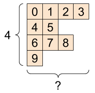
ただ、tensorの各次元へのデータの入れ方の順序は意識していたほうがいいかなと思いました。末尾の次元から特徴量、先頭の次元ではバッチのまとまりのように帯域的なデータのまとまりを保存するようです。

Indexing
ここもNumPyの知識があればほとんど問題ありません。
Single-axis indexing
Multi-axis indexing
Manipulation shapes
ここもNumPyの知識があればほとんど問題ありません。
ただ、次元の転置をするときはtf.reshapeでは行えませんので、tf.transposeを実行する必要があります。
More on DTypes
tv.cast関数を使ってdtypeを変えられるよというお話です。
Broadcasting
tensor同士の演算のbroadcastの話です。 ここもNumPyの知識があればほとんど問題ありません。
tf.convert_to_tonsor
大体のopsはtensorではない引数に対してtf.convert_to_tensor関数を呼び出してtensorに変換するのでtensorではない引数もopsで計算できてしまうようです。
Ragged Tensors
通常のtensorでは以下のような構造のtensorを作成することができません。
このように、ある次元の長さが不規則なtensorを作成するためにtf.RaggedTensorというクラスがあります。
String tensors
文字を扱うtensorもありますが、TensorFlowの概要を理解するのには後回しでいいでしょう。必要になったら戻ってきましょう。
Sparse tensors
以下のように、一部にしかデータが入っておらず、他は0のようなtensorを扱うためにsparse tensorがあります。
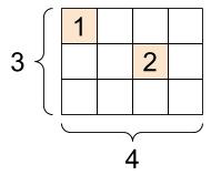
メモリの効率が良かったりするのでしょうか?
まとめ
tensorは大体NumPyのndarrayと思っておけば大丈夫そうです。もっと細かい調整が必要なら詳しく調べてみるくらいのスタンスで初めはいいのではないでしょうか。
Variable
variableはtf.Variableクラスのオブジェクトで、
- opsを実行することで値を更新することができるtensorと考えられる。値を更新することができないtensorとは対照的。
tf.kerasなどの高レベルのライブラリはモデルのパラメータをtf.Variableを使って管理する
のような特徴があります。
Create a variable
variableは
my_tensor = tf.constant([[1.0, 2.0], [3.0, 4.0]])
my_variable = tf.Variable(my_tensor)
のように作成します。
variableはtensorと同じようなメソッドも使えます。ただし、reshapeは新しいtensorを作り出し、元のvariableは更新されません。
また、以下のようにvariableから新しいvariableを作成した際に、bには新しいメモリが割り当てられて、aとメモリを共有していません。ハードコピーというイメージでいい気がします。
a = tf.Variable([2.0, 3.0])
# Create b based on the value of a
b = tf.Variable(a)
Lifecycles, naming, and watching
variableには名前をつけることもできます。
特に、モデルのなかのvariableは保存、読み込み時に名前が保たれます。モデルの中のvariableの名前は一意である必要がありますが、モデルの作成時に自動的に割り当てられるらしいので特に意識する必要はありません。
モデルの中には訓練する必要のないvariableも存在します。そのようなvariableはtrainable=Falseを指定して作成します。
Placing variables and tensors
CPUで計算するかGPUで計算するかなどのお話です。TensorFlowの概要を理解するのには飛ばしていいでしょう。必要になったら戻ってきて理解しましょう。
まとめ
variableとは
- 更新可能なtensorのようなもの
- 特に、Kerasなどではmodelのパラメータにvariableが使われている
- 訓練の必要がないvariableには
trainable=Falseを指定する
です。
Automatic differentiation
この章はTensorFlowの概要を理解するためにはやや高度な話も含まれていたので結構省略してまとめています。
Gradient tapes
TensorFlowは自動微分を計算するためにtf.GradientTape というAPIを用意しています。
tf.GradientTape コンテキスト内で実行される演算を”テープ”に記録し、これらを使って逆伝搬により微分を計算します。
詳しい使い方はサイトを参照してください。
Gradients with respect to a model
tf.Modelを使った演算の自動微分も計算することができますよとのことです。
tf.Modelは別の章で解説されます。
Controlling what the tape watches
自動微分のデフォルトの挙動は訓練可能なtf.Variableにアクセスした後にopsの記録をします。これは
- テープは逆伝搬で微分を計算する際に、どのopsを順伝搬に記録するかを知る必要がある
- 中間出力を保持する必要のないopsがある
- 最も一般的な使い方が、trainable variableに関するモデルの損失の微分を計算することである
のような理由からだそう。
微分が計算できないものとして
tf.Tensortrainable=Falseとなっているtf.Variable
があります。
ただし、tensorの微分を計算するために、GradientTape.watch(x)メソッドが用意されています。
まとめ
tf.GradientTapeは基本的にはtf.Variableの微分を計算するものとひとまず覚えておきましょう。詳しい使い方は少しずつ覚えていきましょう。
Intro to graphs and functions
Overview
What are graphs?
今までの解説はeager executionのもとで実行していました。
eager executionと対になる概念としてgraph executionがあります。graph executionは
- Python以外へのデプロイが可能
- より良いパフォーマンス
などの特徴があります。
graph executionとはtensorの計算をtf.Graphとして実行することです。(そのまんまですね・・・)
graphとはtf.Operationとtf.Tensorをまとめたデータ構造のことです。
The benefits of graphs
graphの利点として、
- saved modelsによりPython以外の環境へエクスポートすることができる
性能面として
- 定数ノードをfoldingすることでtensorの値を静的に解析する(知識不足のため理解できていません・・・)
- 独立した計算を別々のスレッドやデバイスに分割する
- 共通している部分式を削除することで算術演算を簡素化する
などがあります。簡単にいうと、graphはTensorFlowの実行を高速化、並列化します。
Taking advantage of graphs
graphはtf.functionを使って作成します。もしくは、関数定義時にtf.functionをデコレータとして使用することで作成できます。
Converting Python functions to graphs
関数定義にif-then、ループ、breakなどなどのPython構文が含まれている関数をgraph化する際には追加の処理が必要になる可能性があるそうです。
大抵の場合はあまり気にすることはないそうですが、より詳細にはtf.function guideとcomplete AutoGraph referenceを読むと良いそうです。
Polymorphism: one Function, many graphs
一つのFunctionでも、引数のdtypeとshapeごとに新しいtf.Graphを内部的に作成します。各tf.Graphのdtypeとshapeのことをinputo signatureとかsignatureと呼ぶそうです。このように、dtypeとshapeごとにtf.Graphを作成することで最適化されるようです。
Using tf.function
tf.functionをただ使用するだけでgraphを作成できますが、いくつか注意する挙動をここでは紹介しています。
Graph execution vs. eager execution
細かい話なのでリンク先参照でいいでしょう。graphが新しく作成される際のtraceという処理はパフォーマンスの点で重要になります。
tf.function best practices
想定通りにgraph化するためのベストプラクティスとして以下のようなものがあります:
- eager executionとgraph executionを頻繁に切り替えて動作に違いがないかを確認する。
tf.Variableの作成はPythonの関数定義の外側で行い、変更を関数内で行う。これはkeras.layer、keras.Model、tf.optimizerなどにも当てはまる。tf.VariableとKerasのオブジェクト以外に、外部のPython変数に依存する関数を作らない。- 引数はtensorやその他のTensorFlowのオブジェクトにする。それ以外を引数にする際には注意する。
- パフォーマンスの面から、なるべく多くの計算を
tf.functionにまとめる。
Seeing the speed-up
高速化の実例があります。リンク先参照してください。
Performance and trade-offs
graphの作成によるtraceのオーバーヘッドが酷いとパフォーマンスに影響がありますよという話です。
When is a Function tracing?
traceは引数に渡すpythonのオブジェクトが変わるだけで実行されるので注意というお話です。
まとめ
graph executionの特徴として
- Python以外の環境へデプロイすることができるようになる
- eager executionよりもパフォーマンスが良い
- input signature毎に新しいgraphが作成される
- traceのオーバーヘッドによるパフォーマンスの低下に気をつける
を覚えておきましょう。
Intro to modules, layers, and models
modelとは
もののことです。
Defining models and layers in TensorFlow
modelのほとんどはlayerから作られています。layerは再利用可能で、トレーニング可能なvariableを持つ関数です。(再利用可能のニュアンスが不明です・・・)Kerasなどの高レベルのlayerの実装はtf.Moduleのサブクラス化で作られています。
tf.Moduleをサブクラス化した場合、tf.Variableなどは自動的にこのオブジェクトによって収集されて、トレーニングなどにより更新できるようになります。tf.Variableだけではなく別のtf.Moduleのtf.Variableも同様に収集されます。つまり、tf.Moduleはネストできるということです。
Waiting to create variables
特徴量の数が正確に定まっていない時など、入力するtensorの形状が定まっていない場合に、modelの作成時に入力tensorの形状を保留することができるようなこともできますよというお話。
Saving weights
tf.Moduleは保存機能もあるよというお話。
ここではcheckpointという機能を使ってmodelのweight (トレーニングしたvariable)の保存を紹介しています。
Saving functions
Creating a SavedModel
graph化しておけばtf.saved_model.saveを使ってシリアライズすることができますというお話です。
Keras models and layers
Keras layers
tf.keras.layers.Layerはtf.Moduleを継承していて、全てのKeras layerの基底クラスになっています。
tf.keras.layers.Layerを継承するときは__call__をcallにするだけでtf.Moduleの継承と同じように使用することができます。
The build step
入力する特徴量の数をクラスの定義時には定めなくても良くなる仕組みとしてbuildメソッドがあります。
Keras models
tf.keras.layers.Layerよりも機能が豊富なtf.keras.Modelというクラスもあります。使い方はほとんどtf.keras.layers.Layerと同じです。
また、以下のように、関数型を呼び出すようにAPIを使えば、既存のlayerの組み合わせなどのような単純なモデルを作るときは非常に短いコードで作成することができます。
inputs = tf.keras.Input(shape=[3,])

x = FlexibleDense(3)(inputs)
x = FlexibleDense(2)(x)

my_functional_model = tf.keras.Model(inputs=inputs, outputs=x)
Saving Keras models
Kerasのモデルも保存することができますが、別のところで詳しく解説されているので後でいいでしょう。
まとめ
modelとは
- tensorの計算をする(順伝搬)
- トレーニングに応じてvariableの更新ができる
- ほとんどのmodelはlayerからできている
- layerは訓練可能なvariableを持つ数学的な演算を行う関数のこと
- layerは
tf.Moduleを継承することで作成する - 保存機能もある
- Kerasでもmodelと似たようなものを扱える
- Kerasでは
tf.keras.layers.Layerクラスを継承することでmodelを作成する
のような特徴があります。
Training loops
ここでは、今まで紹介してきたtensor、variable、gradient tapeそしてmoduleを使ってモデルをトレーニングする方法を紹介します。
Solving machine learning problems
機械学習の問題を特には通常以下のステップがあります:
- データの入手
- モデルの定義
- 損失関数の定義
- トレーニングデータからの損失関数の計算
- 損失関数の勾配の計算とモデルの重さのデータへのフィット
- 結果の評価
Data
一次関数に正規分布のノイズが加えられたデータの生成です。
Define the model
tf.Moduleを継承して、variableとtensorの計算をカプセル化します。
Define a loss function
損失関数を定義します。ここではL2損失を定義します。
Define a training loop
ここでは、順伝搬を計算して重みを更新するtrain関数と、各エポック毎に損失と重みの更新を記録するtraining_loop関数を定義して、簡単な機械学習モデルの訓練の例を示しています。
The same solution, but with Keras
上でやってきたことを今度はKerasを使って実装します。
Kerasを使うと
train関数とtraining_loop関数のような、訓練を実行する関数を書く必要がない- その代わり、
compileメソッドとfitメソッドを使えば同じことができる compileはoptimizerと損失関数を設定するfitでエポックとバッチサイズを指定して訓練する
のようになります。非常に簡単に書けます。
まとめ
モデルの訓練にはKerasのcompileとfitを使うと簡単に実装できます。
TensorFlow basicsの残りの部分
TensorFlow basicsのこれ以降の部分はTensorFlowの概要を掴むにはやや高度な部分な気がするので、この後はKerasの説明を読むと良いと思います。実際にmodelを作成し始めたらさらに読んでみると良いと思います。
Keras
The Sequential model
ここではKerasのmodelの作り方のうち、sequential modelと呼ばれる方法を紹介します。sequential modelと対になる方法としてfunctional APIと呼ばれる方法があります。それは次の章で解説します。
When to use a Sequential model
sequential modelは一つのtensorを受け取り一つのテンソルを出力する層の単純な積み重ねになっているmodelの作成に適しています。
sequential modelは以下のようにkeras.Sequentialを使用して作成します。
# Define Sequential model with 3 layers
model = keras.Sequential(
    [
        layers.Dense(2, activation="relu", name="layer1"),
        layers.Dense(3, activation="relu", name="layer2"),
        layers.Dense(4, name="layer3"),
    ]
)
ただし、sequential modelが適さない場合として、
などなどの場合には適さないようです。この場合は次の章で紹介するfunctional APIを使用します。
Creating a Sequential model
ここでは色々な方法でsequential modelを作成しています。
Pythonのリストのように、pop、addのようなメソッドで編集することもできるようです。
Specifyng the input shape in advance
keras.Inputオブジェクトを使うと、sequential modelを編集しながらsummaryメソッドでmodelの変数を確認することができるようになります。
A common debugging workflow: add() + summary()
summaryを確認しながらaddでlayerを追加してmodelを作成する例が紹介されています。
What to do once you have a model
model作成後の作業についてのリンクです。guide to multi-GPU and distributed trainingは実際に使う際にGPUの使い方で参考になるかもしれません。
Feature extraction with a Sequential model
中間層からの出力をアウトプットする方法が紹介されていますが、いまいち意図がわかっていません・・・Functional API modelを参考とのことです。
もしかしたら、中間層からの出力を使ってより複雑なmodelを作成することができるって言いたいのかもしれません。
Transfer learning with a Sequential model
特定のlayerの訓練を禁止する方法が紹介されています。また、すでに学習したmodelを使って新たなモデルを作る方法も紹介されています。
まとめ
sequential modelはKerasでmodelを作成する方法の一つで、一つのインプットを入力し一つのアウトプットを出力するlayerの単純な積み重ねのmodelを作成することができます。sequential modelと対になる概念がfunctional APIで、次の章で説明します。
The Functional API
Introduction
sequentialでも言及したように、functional APIはKerasでmodelを作る方法のもう一つの方法です。sequentialよりも複雑なトポロジーを持つmodelを作成することができます。
functional APIの使い方としては、以下のように、各layerを関数のように呼び出してtensorの計算を定めていきます。
inputs = keras.Input(shape=(784,))
dense = layers.Dense(64, activation="relu")
x = dense(inputs)
x = layers.Dense(64, activation="relu")(x)
outputs = layers.Dense(10)(x)
model = keras.Model(inputs=inputs, outputs=outputs, name="mnist_model")
Training, evaluation, and inference
訓練などにはcompile、fit、evaluateなどのメソッドが今までと同様に使えます。
Save and serialize
save()を呼び出せばmodelをシリアライズ化できます。詳しくはSave and load Keras modelsを見ましょう。
Use the same graph of layers to define multiple models
この例では、encoder_inputからencoder_outputを計算するencoderというmodelを作っていますが、さらに、encoder_outputを別のlayerの入力として使いdecoder_outputを計算しています。
出力の使い回しができる感じでしょうか。
All models are callable, just like layers
作成したmodelを別のモデルのlayerとして使用することもできるというお話ですね。
Manipulate complex graph topologies
Models with multiple inputs and outputs
こんな複雑なトポロジーを持つmodelも作れますよというお話。sequential modelではできません。

A toy ResNet model
ResNetのトポロジーも実現できますよというお話。これもsequential modelではできません。
Shared layers
同じlayerを使い回すこともできますよというお話。
Extract and reuse nodes in the graph of layers
中間層の出力もmodelの出力にできるというというお話ですかね?neural style transferをよく知りませんのであまり使い所が分かりませんが。
Extend the API using custom layers
Keralに用意されているlayer以外にも自作のlayerを作成してmodelを作ることができますよというお話です。詳しくはcustom layers and modelsを参照してください。
When to use the functional API
keras.Modelのサブクラス化とfunctional APIの使い分けについて解説しています。より詳しくはWhat are Symbolic and Imperative APIs in TensorFlow 2.0?
を参照してください。ここでは簡単な違いのみ紹介しています。
Functinal API strengths:
まず、作成が簡単という点が挙げられます。keral.Modelのサブクラス化はsuper(MLP, self).__init__(**kwargs)などを書かなければいけないので冗長なコードになります。
次にmodelの検証が簡単らしいです。functional APIは作成中にエラーがあれば随時気がつくことができるのでmodelができればちゃんと動くことが保証されるようなイメージでしょうか。
次に、ここでも見たように、中間layerの出力を確認することができます。
最後に、シリアライズ化することもできます。
Functional API weakness:
functional APIではトポロジーは有向非巡回グラフになるように定義しなければいけないようですが、これだとRNNの実装ができません。keras.Modelのサブクラス化だとRNNの実装ができるそうです。
Mix-and-match API styles
上で、modelの作成方法の優劣について説明しましたが、結局、それらは大した問題にはなりませんというお話です。
functional APIでもkeras.Modelのサブクラス化したmodelをlayerとして使えますし、その逆もできますというお話です。
まとめ
functional APIはmodelを作成する方法の一つで、
- sequential modelよりも柔軟なmodelを作ることができる
- シリアライズ化できる
keras.Modelのサブクラス化と使い分けてより良いmodelを作ることができる
などの特徴があります。
前の章で紹介したsequential modelがいつの間にかfunctional APIの下位互換になったような気がするのですが気のせいでしょうか・・・sequential modelの優位性って何かありましたっけ?
Training and evaluation with the built-in methods
Introduction
ここでは、Model.fit()、Model.evaluate()、Model.predict()の使い方を説明します。
この章はKerasの概要を掴むという意味ではやや高度な話なので飛ばすか、流し見でいいと思います。必要になったら戻ってきましょう。
より詳しいリンクもあるみたいですので、概要を掴んだ後に読んでみると良いでしょう。
API overview: a first end-to-end example
訓練のためにmodelに与えるデータは、メモリに乗り切るならNumPy arrayか、そうでなければtf.dataオブジェクトで渡します。
ここでのコードの例は
- function API でmodelを作って
- mnistデータの取得、前処理
compileでオプティマイザーと損失関数と評価指標の設定fitによる訓練historyによる訓練の履歴取得evaluateによる評価とpredictによる予測
をやっています。今までのおさらいの部分もあるでしょうがKerasによる訓練の流れをざっくり掴むことができます。
The compile() method: specifying a loss, metrics and an optimier
fitにより訓練するためにcompleでオプティマイザーと損失関数を指定する必要があります。評価指標は指定しなくても良いそうです。
Custom losses
損失関数を自作することもできます。y_trueとy_pred以外の引数を損失関数に渡したい場合はtf.keras.losses.Lossをサブクラス化して新しい損失関数のクラスを作成するようです。
Custom metrics
評価指標も自作できますよというお話です。
Handling losses and metrics that don't fit the standard signature
Handling losses and metrics that don't fit the standard signature
modelの重みなどにL2正則化を適用するなど、y_pred以外の値を損失関数に渡す場合はadd_lossメソッドを使うようです。
他にもいろいろ説明されているので余裕ができたら読みましょう。
Automatically setting apart a validation holdout set
訓練データ中の検証データの量を指定するvalidation_splitという引数が紹介されています。
Training & evaluation from tf.data Datasets
今まではmodelにNumPy arrayを渡す例を見てきましたが、ここからはtf.data.Datasetオブジェクト形式で渡す例を見ていきます。
より詳しくはtf.data documentationを参照しましょう。
tf.data.Datasetを使うと、
- 訓練集合のシャッフル
- バッチの指定
- 各エポックで使用するバッチの数
などを指定できるようになったりするそうです。
ただ、NumPy arrayの時はvalidation_splitが使えましたが、tf.data.Datasetの時は使えないようです。
Other input formats supported
modelへの入力として何を使えばいいか迷った際は
- データがメモリに載るくらい小さければNumPy array
- データが大きく、さらに並列で訓練したい場合は
Dataset - データが大きく、Python側で多くの前処理が必要な場合は
keras.utils.Sequence
を意識すると良いそうです。
Using a keras.utils.Sequence object as input
keras.utils.Sequenceの使い方が紹介されています。必要になったら読みましょう。
Using sample weighting and class weighting
サンプルやクラスに重みをつける方法が紹介されています。必要になったら読みましょう。
Passing data to multi-input, multi-output models
複数の入力や複数の出力を扱う場合の方法が説明されています。必要になったら読みましょう。
Using Callbacks
訓練中の特定のタイミングで指定した処理をする仕組みとしてcallbackが用意されています。例えば、早期終了をするcallbackがあります。
他にはcallbacks documentationを読みましょう。
また、callbackも自作できるようです。
Checkpointing models
比較的時間のかかる訓練の途中でcheckpointを保存する仕組みもあります。
詳しくはguide to saving and serializing Modelsを見ましょう。
Using learning rate schedules
訓練が進むにつれて学習率を減少させる機能も用意されているようです。
Visualizing loss and metrics during training
TensorBoardを使うと訓練中の様子を可視化することができるようです。
まとめ
この章ではより柔軟なmodelの構築や訓練の方法などを見ました。実際にKerasを使って複雑なmodelを作る際に参考になりそうです。
Making new Layers and Models via subclassing
この章はKerasの概要を掴むためにはやや高度なので飛ばしてもいいでしょう。必要になったら戻ってきましょう。
ただ、ModelとLayerの違いについてだけ確認しておきます。
The Model class
ModelクラスはLayerクラスと同じようなAPIを持っていますが、加えて以下の特徴があります:
- 訓練、評価、予測用の
model.fit、model.evaluate、model.predictメソッド - 内部のlayerを確認するための
model.layerメソッド - シリアライズ化するための
save、save_weightsメソッド
基本的には、内部的な処理はLayerを使い、それらをまとめて一つのmodelにするときにはModelを使うようです。
Save and load Keras models
この章ではmodelの保存について解説していますが、ひとまず以下のmodelの保存と読み込みを覚えておけばよさそうです。
- 保存:
model = ...  # Get model (Sequential, Functional Model, or Model subclass)
model.save('path/to/location')
- 読み込み
from tensorflow import keras
model = keras.models.load_model('path/to/location')
Working with preprocessing layers
Keras preprocessing layers
Kerasには前処理をするためのLayyerが用意されています。
これらのLayerを使うことで生のデータをそのまま入力できるmodelを作ることができます。
Available preprocessing layers
ここでは、用途毎にさまざまな前処理layerが紹介されています。
残りの部分
この章の残りは必要になってから読めばいいでしょう。
Customize what happens in Model.fit
この章では、fitのオーバーライトをするようですが、高度な話なので必要になったら読めばいいでしょう。
Writing a training loop from scratch
この章では前の章よりもより深くmodelをカスタマイズするようです。これも必要になったら読めば良いでしょう。
終わり
TensorFlowのGuideを読んでみて、TensorFlowの概要を理解するために知っておけばいいと思った箇所は以上になります。
ただ、これ以外にも基本的なクラスはたくさんあります。それらは実際に使い始めて必要になったら読み返せばいいでしょう。
Python 機械学習プログラミング 達人データサイエンティストによる理論と実践 第3章 写経
目次
- 目次
- 始めに
- 3 分類問題ー機械学習ライブラリscikit-learnの活用
始めに
この記事では、[第2版]Python 機械学習プログラミング 達人データサイエンティストによる理論と実践

の3章を写経した記録をまとめます。前回はこちらPython 機械学習プログラミング 達人データサイエンティストによる理論と実践 第2章 写経。 実行はJupyter Labにて実行しています。
写経は以下のようにまとめました。
写経ではありますが、関数を作成し、コードの再実行をやりやすいようにした部分があります。
より良いと思われるコードを考えた場合は書き換えてコメントを添えるようにし、変更点をなるべく明示するようにしてあります。
個人的に気になった点のメモを残すようにしてあります。同じような疑問を持った方の助けになれば幸いです。
以前書いたコードと同じようなコード(例えばグラフの描写等)は効率化のために飛ばしているところもあります。
記事内で使用するモジュールなどは一番最初に宣言するようにしてあります。
[第2版]Python 機械学習プログラミング 達人データサイエンティストによる理論と実践を読んでいている際のちょっとした正誤表代わりになればと思います。
3 分類問題ー機械学習ライブラリscikit-learnの活用
使用モジュール
from sklearn import datasets
import numpy as np
from sklearn.model_selection import train_test_split
from sklearn.preprocessing import StandardScaler
from sklearn.linear_model import Perceptron
from sklearn.metrics import accuracy_score
from matplotlib.colors import ListedColormap
import matplotlib.pyplot as plt
from IPython.core.pylabtools import figsize
from sklearn.linear_model import LogisticRegression
from sklearn.svm import SVC
from sklearn.tree import DecisionTreeClassifier
from sklearn.ensemble import RandomForestClassifier
from sklearn.neighbors import KNeighborsClassifier
3.2 scikit-learnの活用へのファーストステップ:パーセプトロンのトレーニング
iris = datasets.load_iris()
X = iris.data[:, [2, 3]]
y = iris.target

print('Class labels:', np.unique(y))
Class labels: [0 1 2]
メモ(sklearn.utils.Bunchオブジェクトについて)
irisはklearn.utils.Bunchというクラスのインスタンスになっています。
type(iris)
Output:
sklearn.utils.Bunch
klearn.utils.Bunchは辞書に似ているオブジェクトで、アトリビュートによってデータを取り出すことができます。以下に簡単な使い方を紹介しておきます。
import sklearn.utils
以下のようにklearn.utils.Bunchインスタンスを作成します。以下では、キーaに1をキーbに2を所持するklearn.utils.Bunchインスタンスを作成します。
bunch = sklearn.utils.Bunch(a=1, b=2)
通常の辞書のように、コンストラクタで指定したキーの文字列によりデータにアクセスることができます。
bunch['a']
Output:
1
アトリビュートとしてもデータにアクセスすることができます。
bunch.b
Output:
2
新しいキーをとバリューを追加することもできます。
bunch.c = 3
bunch['c']
Output:
3
X_train, X_test, y_train, y_test = train_test_split(
    X, y, test_size=0.3, random_state=1, stratify=y)
print('Labels counts in y:', np.bincount(y))
print('Labels counts in y_train:', np.bincount(y_train))
print('Labels counts in y_test:', np.bincount(y_test))
Output:
    Labels counts in y: [50 50 50]
    Labels counts in y_train: [35 35 35]
    Labels counts in y_test: [15 15 15]
sc = StandardScaler()
sc.fit(X_train)
X_train_std = sc.transform(X_train)
X_test_std = sc.transform(X_test)
ppn = Perceptron(max_iter=40, eta0=0.1, random_state=1) # n_iterは今後削除される予定であるというwarningが出た。n_iterはmax_iterに引き継がれたよう。
ppn.fit(X_train_std, y_train)
Output:
    Perceptron(alpha=0.0001, class_weight=None, early_stopping=False, eta0=0.1,
          fit_intercept=True, max_iter=40, n_iter=None, n_iter_no_change=5,
          n_jobs=None, penalty=None, random_state=1, shuffle=True, tol=None,
          validation_fraction=0.1, verbose=0, warm_start=False)
y_pred = ppn.predict(X_test_std)
print('Misclassified samples: %d' % (y_test != y_pred).sum())
Output:
Misclassified samples: 9
print('Accuracy: %.2f' % accuracy_score(y_test, y_pred))
Output:
Accuracy: 0.80
print('Accuracy: %.2f' % ppn.score(X_test_std, y_test))
Output:
Accuracy: 0.80
def plot_decision_regions(X, y, classifier, test_idx=None, resolution=0.02):
    markers = ('s', 'x', 'o', '^', 'v')
    colors = ('red', 'blue', 'lightgreen', 'gray', 'cyan')
    cmap = ListedColormap(colors[:len(np.unique(y))])

    x1_min, x1_max = X[:, 0].min() - 1, X[:, 0].max() + 1
    x2_min, x2_max = X[:, 1].min() - 1, X[:, 1].max() + 1
    xx1, xx2 = np.meshgrid(np.arange(x1_min, x1_max, resolution),
                           np.arange(x2_min, x2_max, resolution))
    Z = classifier.predict(np.array([xx1.ravel(), xx2.ravel()]).T)
    Z = Z.reshape(xx1.shape)
    plt.contourf(xx1, xx2, Z, alpha=0.3, cmap=cmap)
    plt.xlim(xx1.min(), xx1.max())
    plt.ylim(xx2.min(), xx2.max())

    for idx, cl in enumerate(np.unique(y)):
        plt.scatter(x=X[y == cl, 0],
                    y=X[y == cl, 1],
                    alpha=0.8,
                    c=colors[idx],
                    marker=markers[idx],
                    label=cl,
                    edgecolor='black')

    if test_idx:
        X_test, y_test = X[test_idx, :], y[test_idx]

        plt.scatter(X_test[:, 0],
                    X_test[:, 1],
                    c='',
                    edgecolor='black',
                    alpha=1.0,
                    linewidth=1,
                    marker='o',
                    s=100,
                    label='test set')
X_combined_std = np.vstack((X_train_std, X_test_std))
y_combined = np.hstack((y_train, y_test))

figsize(10, 7)
plt.rcParams['font.size'] = 20

plot_decision_regions(X=X_combined_std, y=y_combined,
                      classifier=ppn, test_idx=range(105, 150))
plt.xlabel('petal length [standardized]')
plt.ylabel('petal width [standardized]')
plt.legend(loc='upper left')

plt.tight_layout()
plt.show()

3.3.3 ADALINE実装をロジスティック回帰のアルゴリズムに変換する
class LogisticRegressionGD(object):
    def __init__(self, eta=0.05, n_iter=100, random_state=1):
        self.eta = eta
        self.n_iter = n_iter
        self.random_state = random_state

    def fit(self, X, y):
        rgen = np.random.RandomState(self.random_state)
        self.w_ = rgen.normal(loc=0.0, scale=0.01, size=1 + X.shape[1])
        self.cost_ = []

        for i in range(self.n_iter):
            net_input = self.net_input(X)
            output = self.activation(net_input)
            errors = (y - output)
            self.w_[1:] += self.eta * X.T.dot(errors)
            self.w_[0] += self.eta * errors.sum()
            cost = -y.dot(np.log(output)) - ((1 - y).dot(np.log(1 - output)))
            self.cost_.append(cost)
        return self

    def net_input(self, X):
        return np.dot(X, self.w_[1:]) + self.w_[0]

    def activation(self, z):
        return 1. / (1. + np.exp(-np.clip(z, -250, 250)))

    def predict(self, X):
        return np.where(self.net_input(X) >= 0.0, 1, 0)
X_train_01_subset = X_train[(y_train == 0) | (y_train == 1)]
y_train_01_subset = y_train[(y_train == 0) | (y_train == 1)]

lrgd = LogisticRegressionGD(eta=0.05, n_iter=1000, random_state=1)
lrgd.fit(X_train_01_subset,
         y_train_01_subset)

plot_decision_regions(X=X_train_01_subset,
                      y=y_train_01_subset,
                      classifier=lrgd)

plt.xlabel('petal length [standardized]')
plt.ylabel('petal width [standardized]')
plt.legend(loc='upper left')

plt.tight_layout()

3.3.4 scikit-learnを使ったロジスティック回帰モデルのトレーニング
lr = LogisticRegression(C=100.0, random_state=1, solver='liblinear', multi_class='ovr') # solverとmulti_class引数を明示的に指定しないとwarningが出力された。
lr.fit(X_train_std, y_train)

plot_decision_regions(X_combined_std, y_combined,
                      classifier=lr, test_idx=range(105, 150))
plt.xlabel('petal length [standardized]')
plt.ylabel('petal width [standardized]')
plt.legend(loc='upper left')
plt.tight_layout()
plt.show()

3.4 サポートベクトルマシンによる最大マージン分類
3.4.2 スラック変数を使った線形分離不可能なケースへの対処
svm = SVC(kernel='linear', C=1.0, random_state=1)
svm.fit(X_train_std, y_train)

plot_decision_regions(X_combined_std,
                      y_combined,
                      classifier=svm,
                      test_idx=range(105, 150))
plt.xlabel('petal length [standardized]')
plt.ylabel('petal width [standardized]')
plt.legend(loc='upper left')
plt.tight_layout()
plt.show()

3.5 カーネルSVMを使った非線形問題の求解
3.5.1 線形分離不可能なデータに対するカーネル手法
np.random.seed(1)
X_xor = np.random.randn(200, 2)
y_xor = np.logical_xor(X_xor[:, 0] > 0,
                       X_xor[:, 1] > 0)
y_xor = np.where(y_xor, 1, -1)

plt.scatter(X_xor[y_xor == 1, 0],
            X_xor[y_xor == 1, 1],
            c='b', marker='x',
            label='1')
plt.scatter(X_xor[y_xor == -1, 0],
            X_xor[y_xor == -1, 1],
            c='r',
            marker='s',
            label='-1')

plt.xlim([-3, 3])
plt.ylim([-3, 3])
plt.legend(loc='best')
plt.tight_layout()
plt.show()

svm = SVC(kernel='rbf', random_state=1, gamma=0.10, C=10.0)
svm.fit(X_xor, y_xor)
plot_decision_regions(X_xor, y_xor,
                      classifier=svm)

plt.legend(loc='upper left')
plt.tight_layout()
plt.show()

svm = SVC(kernel='rbf', random_state=1, gamma=0.2, C=1.0)
svm.fit(X_train_std, y_train)

plot_decision_regions(X_combined_std, y_combined,
                      classifier=svm, test_idx=range(105, 150))
plt.xlabel('petal length [standardized]')
plt.ylabel('petal width [standardized]')
plt.legend(loc='upper left')
plt.tight_layout()
plt.show()

svm = SVC(kernel='rbf', random_state=1, gamma=100.0, C=1.0)
svm.fit(X_train_std, y_train)

plot_decision_regions(X_combined_std, y_combined,
                      classifier=svm, test_idx=range(105, 150))
plt.xlabel('petal length [standardized]')
plt.ylabel('petal width [standardized]')
plt.legend(loc='upper left')
plt.tight_layout()
#plt.savefig('images/03_16.png', dpi=300)
plt.show()

3.6 決定木学習
3.6.2 決定木の構築
tree = DecisionTreeClassifier(criterion='gini',
                              max_depth=4,
                              random_state=1)
tree.fit(X_train, y_train)

X_combined = np.vstack((X_train, X_test))
y_combined = np.hstack((y_train, y_test))
plot_decision_regions(X_combined, y_combined,
                      classifier=tree, test_idx=range(105, 150))

plt.xlabel('petal length [cm]')
plt.ylabel('petal width [cm]')
plt.legend(loc='upper left')
plt.tight_layout()

plt.show()

3.6.3 ランダムフォレストを使って複数の決定木を結合する
forest = RandomForestClassifier(criterion='gini',
                                n_estimators=25,
                                random_state=1,
                                n_jobs=2)
forest.fit(X_train, y_train)

plot_decision_regions(X_combined, y_combined,
                      classifier=forest, test_idx=range(105, 150))

plt.xlabel('petal length [cm]')
plt.ylabel('petal width [cm]')
plt.legend(loc='upper left')
plt.tight_layout()

plt.show()

3.7 k近傍法:怠惰学習アルゴリズム
knn = KNeighborsClassifier(n_neighbors=5,
                           p=2,
                           metric='minkowski')
knn.fit(X_train_std, y_train)

plot_decision_regions(X_combined_std, y_combined,
                      classifier=knn, test_idx=range(105, 150))

plt.xlabel('petal length [standardized]')
plt.ylabel('petal width [standardized]')
plt.legend(loc='upper left')
plt.tight_layout()

plt.show()

今回の写経は以上です。 ここまで読んでいただきありがとうございました。
Python 機械学習プログラミング 達人データサイエンティストによる理論と実践 第2章 写経
目次
始めに
この記事では、[第2版]Python 機械学習プログラミング 達人データサイエンティストによる理論と実践
の2章を写経した記録をまとめます。本を選んだ理由はこちら新しく写経する本を紹介(Python 機械学習プログラミング)。 実行はJupyter Labにて実行しています。
写経は以下のようにまとめました。
写経ではありますが、関数を作成し、コードの再実行をやりやすいようにした部分があります。
より良いと思われるコードを考えた場合は書き換えてコメントを添えるようにし、変更点をなるべく明示するようにしてあります。
個人的に気になった点のメモを残すようにしてあります。同じような疑問を持った方の助けになれば幸いです。
以前書いたコードと同じようなコード(例えばグラフの描写等)は効率化のために飛ばしているところもあります。
記事内で使用するモジュールなどは一番最初に宣言するようにしてあります。
[第2版]Python 機械学習プログラミング 達人データサイエンティストによる理論と実践を読んでいている際のちょっとした正誤表代わりになればと思います。
この記事で使用する主なモジュール、設定
この記事では、主に以下のモジュールや設定を使用しています。
2章 分類問題ー単純な機械学習アルゴリズムのトレーニング
使用モジュール
%matplotlib inline
import numpy as np
import pandas as pd
import matplotlib.pyplot as plt
from IPython.core.pylabtools import figsize
from matplotlib.colors import ListedColormap
2.2 パーセプトロンの学習アルゴリズムをPythonで実装する
2.2.1 オブジェクト指向のパーセプトロンAPI
class Perceptron(object):
    def __init__(self, eta=0.01, n_iter=50, random_state=1):
        self.eta = eta
        self.n_iter = n_iter
        self.random_state = random_state

    def fit(self, X, y):
        rgen = np.random.RandomState(self.random_state)
        self.w_ = rgen.normal(loc=0.0, scale=0.01, size=1 + X.shape[1])
        self.errors_ = []

        for _ in range(self.n_iter):
            errors = 0
            for xi, target in zip(X, y):
                update = self.eta * (target - self.predict(xi))
                self.w_[1:] += update * xi
                self.w_[0] += update
                errors += int(update != 0.0)
            self.errors_.append(errors)
        return self

    def net_input(self, X):
        return np.dot(X, self.w_[1:]) + self.w_[0]

    def predict(self, X):
        return np.where(self.net_input(X) >= 0.0, 1, -1)
メモ(np.random.RandomStateクラス)
np.random.RandomStateクラス(numpy.random.RandomState)は確率分布に従う乱数を返すメソッドをいくつか持っています。normalメソッドもそのうちの一つで、正規分布に従う乱数を返します。
rgen = np.random.RandomState(1)
rgen.normal(loc=0.0, scale=0.01, size=5)
Output:
array([ 0.01624345, -0.00611756, -0.00528172, -0.01072969, 0.00865408])
メモ(np.where関数)
上記のコードのnp.where(self.net_input(X) >= 0.0, 1, -1)では、self.net_input(X)の要素が0.0以上なら1を、0.0より小さいなら-1を要素に持つarrayオブジェクトを返します。np.whereのdocstringは以下になります。
np.where??
Output:(クリックすると展開されます)
Docstring:
where(condition, [x, y])

Return elements chosen from `x` or `y` depending on `condition`.

.. note::
    When only `condition` is provided, this function is a shorthand for
    ``np.asarray(condition).nonzero()``. Using `nonzero` directly should be
    preferred, as it behaves correctly for subclasses. The rest of this
    documentation covers only the case where all three arguments are
    provided.

Parameters
----------
condition : array_like, bool
    Where True, yield `x`, otherwise yield `y`.
x, y : array_like
    Values from which to choose. `x`, `y` and `condition` need to be
    broadcastable to some shape.

Returns
-------
out : ndarray
    An array with elements from `x` where `condition` is True, and elements
    from `y` elsewhere.

See Also
--------
choose
nonzero : The function that is called when x and y are omitted

Notes
-----
If all the arrays are 1-D, `where` is equivalent to::

    [xv if c else yv
     for c, xv, yv in zip(condition, x, y)]

Examples
--------
>>> a = np.arange(10)
>>> a
array([0, 1, 2, 3, 4, 5, 6, 7, 8, 9])
>>> np.where(a < 5, a, 10*a)
array([ 0,  1,  2,  3,  4, 50, 60, 70, 80, 90])

This can be used on multidimensional arrays too:

>>> np.where([[True, False], [True, True]],
...          [[1, 2], [3, 4]],
...          [[9, 8], [7, 6]])
array([[1, 8],
       [3, 4]])

The shapes of x, y, and the condition are broadcast together:

>>> x, y = np.ogrid[:3, :4]
>>> np.where(x < y, x, 10 + y)  # both x and 10+y are broadcast
array([[10,  0,  0,  0],
       [10, 11,  1,  1],
       [10, 11, 12,  2]])

>>> a = np.array([[0, 1, 2],
...               [0, 2, 4],
...               [0, 3, 6]])
>>> np.where(a < 4, a, -1)  # -1 is broadcast
array([[ 0,  1,  2],
       [ 0,  2, -1],
       [ 0,  3, -1]])
Type:      builtin_function_or_method
以下のような使い方もできるようです。個人的に、使い方をマスターしておきたい関数です。応用が広がりそうな気がします。
np.where([True, False, True, True],
          [1, 1, 1, 1],
          [0, 0, 0, 0])
Output:
array([1, 0, 1, 1])
2.3 Irisデータセットでのパーセプトロンモデルのトレーニング
df = pd.read_csv('https://archive.ics.uci.edu/ml/'
                 'machine-learning-databases/iris/iris.data', header=None)
df.tail()
Output:
| 0 | 1 | 2 | 3 | 4 | |
|---|---|---|---|---|---|
| 145 | 6.7 | 3.0 | 5.2 | 2.3 | Iris-virginica |
| 146 | 6.3 | 2.5 | 5.0 | 1.9 | Iris-virginica |
| 147 | 6.5 | 3.0 | 5.2 | 2.0 | Iris-virginica |
| 148 | 6.2 | 3.4 | 5.4 | 2.3 | Iris-virginica |
| 149 | 5.9 | 3.0 | 5.1 | 1.8 | Iris-virginica |
メモ(df.tailメソッド)
df.tailメソッドは引数に整数を受け取り、その行数分の末尾のデータを返します。デフォルトでは5行を返すことになっています。
print(df.tail.__doc__)
Output:(クリックすると展開されます)
            Return the last `n` rows.

            This function returns last `n` rows from the object based on
            position. It is useful for quickly verifying data, for example,
            after sorting or appending rows.

            Parameters
            ----------
            n : int, default 5
                Number of rows to select.

            Returns
            -------
            type of caller
                The last `n` rows of the caller object.

            See Also
            --------
            pandas.DataFrame.head : The first `n` rows of the caller object.

            Examples
            --------
            >>> df = pd.DataFrame({'animal':['alligator', 'bee', 'falcon', 'lion',
            ...                    'monkey', 'parrot', 'shark', 'whale', 'zebra']})
            >>> df
                  animal
            0  alligator
            1        bee
            2     falcon
            3       lion
            4     monkey
            5     parrot
            6      shark
            7      whale
            8      zebra

            Viewing the last 5 lines

            >>> df.tail()
               animal
            4  monkey
            5  parrot
            6   shark
            7   whale
            8   zebra

            Viewing the last `n` lines (three in this case)

            >>> df.tail(3)
              animal
            6  shark
            7  whale
            8  zebra
y = df.iloc[0:100, 4].values
y = np.where(y == 'Iris-setosa', -1, 1)

X = df.iloc[0:100, [0, 2]].values

figsize(10, 7)
plt.rcParams['font.size'] = 20
plt.scatter(X[:50, 0], X[:50, 1],
            color='red', marker='o', label='setosa')
plt.scatter(X[50:100, 0], X[50:100, 1],
            color='blue', marker='x', label='versicolor')

plt.xlabel('sepal length [cm]')
plt.ylabel('petal length [cm]')
plt.legend(loc='upper left')

plt.show()
Output:

ppn = Perceptron(eta=0.1, n_iter=10)

ppn.fit(X, y)

plt.plot(range(1, len(ppn.errors_) + 1), ppn.errors_, marker='o')
plt.xlabel('Epochs')
plt.ylabel('Number of updates')

plt.show()
Output:

def plot_decision_regions(X, y, classifier, resolution=0.02):

    markers = ('s', 'x', 'o', '^', 'v')
    colors = ('red', 'blue', 'lightgreen', 'gray', 'cyan')
    cmap = ListedColormap(colors[:len(np.unique(y))])

    x1_min, x1_max = X[:, 0].min() - 1, X[:, 0].max() + 1
    x2_min, x2_max = X[:, 1].min() - 1, X[:, 1].max() + 1
    xx1, xx2 = np.meshgrid(np.arange(x1_min, x1_max, resolution),
                           np.arange(x2_min, x2_max, resolution))
    Z = classifier.predict(np.array([xx1.ravel(), xx2.ravel()]).T) # ravelにより、一次元arrayに変換し、Tにより転置し、predictメソッドが引数として受け取れるように変換している。
    Z = Z.reshape(xx1.shape) # predictメソッドにより予測した結果をreshapeによりxx1らと同じsizeのarrayに変換している。
    plt.contourf(xx1, xx2, Z, alpha=0.3, cmap=cmap)
    plt.xlim(xx1.min(), xx1.max())
    plt.ylim(xx2.min(), xx2.max())

    for idx, cl in enumerate(np.unique(y)):
        plt.scatter(x=X[y == cl, 0],
                    y=X[y == cl, 1],
                    alpha=0.8,
                    c=colors[idx],
                    marker=markers[idx],
                    label=cl,
                    edgecolor='black')
メモ(ravelメソッド)
np.ravleメソッドは引数に渡されたarrayを一次元のarrayに変換します:
np.array([[1, 2], [3, 4]]).ravel()
Output:
array([1, 2, 3, 4])
また、展開する順序を定めるorder引数があります。order引数には'C'、'F'、'A'、'K'のいずれかを設定することができます。デフォルトは'C'です。例えば、'F'を設定すると、列方向に展開します:
np.array([[1, 2], [3, 4]]).ravel(order='F')
Output:
array([1, 3, 2, 4])
figsize(10, 7)
plt.rcParams['font.size'] = 20

plot_decision_regions(X, y, classifier=ppn)
plt.xlabel('sepal length [cm]')
plt.ylabel('petal length [cm]')
plt.legend(loc='upper left')

plt.show()
Output:

2.5.1 ADALINEをPythonで実装する
class AdalineGD(object):
    def __init__(self, eta=0.01, n_iter=50, random_state=1):
        self.eta = eta
        self.n_iter = n_iter
        self.random_state = random_state

    def fit(self, X, y):
        rgen = np.random.RandomState(self.random_state)
        self.w_ = rgen.normal(loc=0.0, scale=0.01, size=1 + X.shape[1])
        self.cost_ = []

        for i in range(self.n_iter):
            net_input = self.net_input(X)
            output = self.activation(net_input)
            errors = (y - output)
            self.w_[1:] += self.eta * X.T.dot(errors)
            self.w_[0] += self.eta * errors.sum()
            cost = (errors**2).sum() / 2.0
            self.cost_.append(cost)
        return self

    def net_input(self, X):
        return np.dot(X, self.w_[1:]) + self.w_[0]

    def activation(self, X):
        return X

    def predict(self, X):
        return np.where(self.activation(self.net_input(X)) >= 0.0, 1, -1)
figsize(20, 7)
plt.rcParams['font.size'] = 20

fig, ax = plt.subplots(nrows=1, ncols=2)

ada1 = AdalineGD(n_iter=10, eta=0.01).fit(X, y)
ax[0].plot(range(1, len(ada1.cost_) + 1), np.log10(ada1.cost_), marker='o')
ax[0].set_xlabel('Epochs')
ax[0].set_ylabel('log(Sum-squared-error)')
ax[0].set_title('Adaline - Learning rate 0.01')

ada2 = AdalineGD(n_iter=10, eta=0.0001).fit(X, y)
ax[1].plot(range(1, len(ada2.cost_) + 1), ada2.cost_, marker='o')
ax[1].set_xlabel('Epochs')
ax[1].set_ylabel('Sum-squared-error')
ax[1].set_title('Adaline - Learning rate 0.0001')

plt.show()
Output:

2.5.2 特徴量のスケーリングを通じて勾配降下法を改善する
X_std = np.copy(X)
X_std[:, 0] = (X[:, 0] - X[:, 0].mean()) / X[:, 0].std()
X_std[:, 1] = (X[:, 1] - X[:, 1].mean()) / X[:, 1].std()
ada = AdalineGD(n_iter=15, eta=0.01)
ada.fit(X_std, y)

figsize(10, 7)
plt.rcParams['font.size'] = 20

plot_decision_regions(X_std, y, classifier=ada)
plt.title('Adaline - Gradient Descent')
plt.xlabel('sepal length [standardized]')
plt.ylabel('petal length [standardized]')
plt.legend(loc='upper left')
plt.tight_layout()
plt.show()

plt.plot(range(1, len(ada.cost_) + 1), ada.cost_, marker='o')
plt.xlabel('Epochs')
plt.ylabel('Sum-squared-error')

plt.tight_layout()
plt.show()
Output:

Output:

class AdalineSGD(object):
    def __init__(self, eta=0.01, n_iter=10, shuffle=True, random_state=None):
        self.eta = eta
        self.n_iter = n_iter
        self.w_initialized = False
        self.shuffle = shuffle
        self.random_state = random_state

    def fit(self, X, y):
        self._initialize_weights(X.shape[1])
        self.cost_ = []
        for i in range(self.n_iter):
            if self.shuffle:
                X, y = self._shuffle(X, y)
            cost = []
            for xi, target in zip(X, y):
                cost.append(self._update_weights(xi, target))
            avg_cost = sum(cost) / len(y)
            self.cost_.append(avg_cost)
        return self

    def partial_fit(self, X, y):
        if not self.w_initialized:
            self._initialize_weights(X.shape[1])
        if y.ravel().shape[0] > 1:
            for xi, target in zip(X, y):
                self._update_weights(xi, target)
        else:
            self._update_weights(X, y)
        return self

    def _shuffle(self, X, y):
        r = self.rgen.permutation(len(y))
        return X[r], y[r]

    def _initialize_weights(self, m):
        self.rgen = np.random.RandomState(self.random_state)
        self.w_ = self.rgen.normal(loc=0.0, scale=0.01, size=1 + m)
        self.w_initialized = True

    def _update_weights(self, xi, target):
        output = self.activation(self.net_input(xi))
        error = (target - output)
        self.w_[1:] += self.eta * xi.dot(error)
        self.w_[0] += self.eta * error
        cost = 0.5 * error**2
        return cost

    def net_input(self, X):
        return np.dot(X, self.w_[1:]) + self.w_[0]

    def activation(self, X):
        return X

    def predict(self, X):
        return np.where(self.activation(self.net_input(X)) >= 0.0, 1, -1)
ada = AdalineSGD(n_iter=15, eta=0.01, random_state=1)
ada.fit(X_std, y)

plot_decision_regions(X_std, y, classifier=ada)
plt.title('Adaline - Stochastic Gradient Descent')
plt.xlabel('sepal length [standardized]')
plt.ylabel('petal length [standardized]')
plt.legend(loc='upper left')

plt.tight_layout()
plt.show()

plt.plot(range(1, len(ada.cost_) + 1), ada.cost_, marker='o')
plt.xlabel('Epochs')
plt.ylabel('Average Cost')

plt.tight_layout()
plt.show()
Output:

Output:

メモ(if y.ravel().shape[0] > 1:の場合分けについて)
コードを見ていて、if y.ravel().shape[0] > 1:の場合分けは必要ないのではと思っていました。しかし、これはこのコードにおいては本質的に必要なようです。どうやら、zipの挙動がy.ravel().shape[0] = 1とy.ravel().shape[0] > 1で異なるために場合分けしているようです。
以下の例によりzipの挙動の違いを見ることができます。まず、yの要素数が1より大きい時は、zipは望んでいる動作をします。
y_value = np.array([1, 1])
X_std[0:2, :]
Output:
    array([[-0.5810659 , -1.01435952],
           [-0.89430898, -1.01435952]])
for xi, target in zip(X_std[0:2, :], y_value):
    print(xi, target)
Output:
    [-0.5810659  -1.01435952] 1
    [-0.89430898 -1.01435952] 1
しかし、yが一つの値しか持たない場合、zipは以下のようなループを実行します。yが値を一つしか含まないようなarrayの場合、zipによりX_std[0, :]からは1行1列目の値が返されます。1行を丸ごと返してはくれません。
y_value = np.array([1])
X_std[0, :]
Output:
array([-0.5810659 , -1.01435952])
for xi, target in zip(X_std[0, :], y_value):
    print(xi, target)
Output:
-0.5810659036233256 1
zipが上記のような動作をするために、if y.ravel().shape[0] > 1:の場合分けが必要になってきます。
今回の写経は以上です。 ここまで読んでいただきありがとうございました。
新しく写経する本を紹介(Python 機械学習プログラミング)
本の紹介
新しく写経していく本を紹介します。新しく写経していく本は [第2版]Python 機械学習プログラミング 達人データサイエンティストによる理論と実践 (impress top gear)
にしました。
選んだ理由
実はもうすでに3章まで写経しているのですが、コードの説明が結構丁寧な印象があって読みやすかったです。
また、機械学習界隈の常識のようなものも注釈などで補足してあって、独学するには良いかなぁと思いました。
今のところの感想
ある程度、アルゴリズムはわかっていて、実装したことない人向けの印象です。PRMLと一緒に読むといいかもしれません。僕はある程度PRMLを読んでいて理論は何となくですがわかっています。そのため、scikit-learnなどのモジュールを使用する部分は、裏でどんなことをしているかがなんとなくわかります。半面、理論を知らないと、scikit-learnなどのモジュールを使用する部分はほぼブラックボックスと化す印象です。理論ってやっぱ重要ですね。
python-twitterモジュールからtwitter APIを使用する方法
目次
目的
この記事では、PythonからtwitterのAPIを操作するためのモジュールであるpython-twitterの基本的な使い方を紹介します。公式ドキュメントは以下になります。
公式ドキュメント:python-twitter
前提条件
この記事では、以下のことに断っておきます。まだまだ勉強不足なことが多く、言葉の使い方などが誤っているかもしれませんがお許しください。
この記事の対象はtwitterでフォローリフォローを自動化したい、Pythonからtwitterの検索結果を取得したいなど、twitterのAPIを個人的に利用したい方向けの記事となります。不特定多数のユーザーに対するアプリケーションを作ることは想定していません。
僕はまだまだ勉強不足なので、実行環境などの詳しい説明ができないということを断っておきます。とりあえず、OSはwindows10で実行しています。Python は3.6.8でした。
既にTwitterのアプリケーションは作成済みで、APi key、APi secret key、Access token、Access token secretの四つを取得済みであることを想定しています。まだの方はTwitter Appからアプリケーションを作成し、各キーを取得しておいてください。
コードの実行はJupyter Labになります。
ただ、初心者の私でもなんとか使用することができたpython-twitterモジュールの日本語での説明があまり見当たらなかったので、少しでも役に立てればと思った次第でこの記事を書きました。
インストール
以下のコマンドでインストールができます。僕はAnaconda Promptから実行しました。コマンドプロンプトからでも実行ができるでしょう。
(base) C:\Users\hoge>pip install python-twitter
インポートとApiインスタンスの作成
python-twitterモジュールのインポートは以下のように行います。名前がpython-twitterなのにインポートはtwitterという名前でインポートするので少し紛らわしいです。
import twitter
APIを使用するにはApiクラスのインスタンスを作成します。このときに、あらかじめ用意した四つのキーが必要になります。アプリケーションの画面から確認してください。

上の画面を参考に、各引数にキーを渡してください。以下は例になります。
api = twitter.Api(consumer_key='kdWcdakeVdDF4PAdKWERTdkekL',
                  consumer_secret='3k22kwkLfN2KKasdeAa2A1aKUIUvbW83S11AaakA123ASDaASD',
                  access_token_key='12344566778890123561aaaaAaasAaA1AAAasAdfHJKklAlA89',
                  access_token_secret='asdGHjkKa1K1asdfgHjK45lASDfHJKklaDasJKlHjDasd',
                 )
apiインスタンスのメソッド
以下に、apiインスタンスメソッドを羅列します。
api.PostUpdates(status)
api.PostDirectMessage(user, text)
api.GetUser(user)
api.GetReplies()
api.GetUserTimeline(user)
api.GetHomeTimeline()
api.GetStatus(status_id)
api.GetStatuses(status_ids)
api.DestroyStatus(status_id)
api.GetFriends(user)
api.GetFollowers()
api.GetFeatured()
api.GetDirectMessages()
api.GetSentDirectMessages()
api.PostDirectMessage(user, text)
api.DestroyDirectMessage(message_id)
api.DestroyFriendship(user)
api.CreateFriendship(user)
api.LookupFriendship(user)
api.VerifyCredentials()
この記事では、いくつかのメソッドを例にしてpython-twitterモジュールの使い方を紹介します。
ユーザーの情報を取得する
ユーザーの情報を取得する方法を紹介します。今回は皆さん大好きのデレステの公式アカウント@imascg_stageさんの情報を取得してみます。

ユーザーの情報を取得するにはapi.GetUserメソッドを使用します。api.GetUserメソッドのscreen_name引数に取得したいユーザーの名前(@でリプライするときに使用する名前)を渡して実行します。
imascg_stage = api.GetUser(screen_name='imascg_stage')
twitter.models.Userという型のインスタンスが生成されます。
type(imascg_stage)
Output:
twitter.models.User
得られた情報はAsDictメソッドにより辞書に変換できます。アカウントのプロフィールやフォロー数、フォロワー数などなどたくさんの情報が見られます。
imascg_stage.AsDict()
Output:
    {'created_at': 'Tue May 19 09:34:46 +0000 2015',
     'description': '「アイドルマスター シンデレラガールズ スターライトステージ」公式アカウントです。※お客様からの個別のメッセージなどは、Twitter上ではご返答できかねますのでご了承下さい。 #デレステ Android:http://t.co/PfCtF9Biv4       iOS:http://t.co/0zb47ZumGb',
     'followers_count': 918550,
     'friends_count': 8,
     'id': 3220191374,
     'id_str': '3220191374',
     'lang': 'ja',
     'listed_count': 10040,
     'name': 'スターライトステージ',
     'profile_background_color': '000000',
     'profile_background_image_url': 'http://abs.twimg.com/images/themes/theme1/bg.png',
     'profile_background_image_url_https': 'https://abs.twimg.com/images/themes/theme1/bg.png',
     'profile_banner_url': 'https://pbs.twimg.com/profile_banners/3220191374/1535901092',
     'profile_image_url': 'http://pbs.twimg.com/profile_images/875515457364557825/zzJa2735_normal.jpg',
     'profile_image_url_https': 'https://pbs.twimg.com/profile_images/875515457364557825/zzJa2735_normal.jpg',
     'profile_link_color': '89C9FA',
     'profile_sidebar_border_color': '000000',
     'profile_sidebar_fill_color': '000000',
     'profile_text_color': '000000',
     'screen_name': 'imascg_stage',
     'status': {'created_at': 'Fri Apr 12 11:06:55 +0000 2019',
      'hashtags': [{'text': '放課後スタジオ'}],
      'id': 1116658954640035842,
      'id_str': '1116658954640035842',
      'lang': 'ja',
      'retweet_count': 430,
      'retweeted_status': {'created_at': 'Fri Apr 05 16:25:58 +0000 2019',
       'favorite_count': 858,
       'hashtags': [{'text': '放課後スタジオ'}],
       'id': 1114202530177622016,
       'id_str': '1114202530177622016',
       'lang': 'ja',
       'retweet_count': 430,
       'source': '<a href="http://twitter.com/download/iphone" rel="nofollow">Twitter for iPhone</a>',
       'text': '【#放課後スタジオ キャンペーン!】\n\n「アイドルマスター シンデレラガールズ U149 放課後スタジオ」を聴くとU149パーカーが抽選で当たるキャンペーンがスタート!\n\n応募締切は【5/13 12時】まで!\n詳細はこちらから⇒… https://t.co/r35dQuZ5yR',
       'truncated': True,
       'urls': [{'expanded_url': 'https://twitter.com/i/web/status/1114202530177622016',
         'url': 'https://t.co/r35dQuZ5yR'}],
       'user_mentions': []},
      'source': '<a href="https://mobile.twitter.com" rel="nofollow">Twitter Web App</a>',
      'text': 'RT @cycomi: 【#放課後スタジオ キャンペーン!】\n\n「アイドルマスター シンデレラガールズ U149 放課後スタジオ」を聴くとU149パーカーが抽選で当たるキャンペーンがスタート!\n\n応募締切は【5/13 12時】まで!\n詳細はこちらから⇒https://t.co/…',
      'urls': [],
      'user_mentions': [{'id': 4023021733,
        'id_str': '4023021733',
        'name': 'サイコミ',
        'screen_name': 'cycomi'}]},
     'statuses_count': 2409,
     'url': 'http://t.co/7REykaZIlX',
     'verified': True}
各情報にアクセスするには辞書で確認したアトリビュートを使用します。たとえば、プロフィールを表示したい場合はdescriptionというアトリビュートを指定します。
imascg_stage.description
Output:
'「アイドルマスター シンデレラガールズ スターライトステージ」公式アカウントです。※お客様からの個別のメッセージなどは、Twitter上ではご返答できかねますのでご了承下さい。 #デレステ Android:http://t.co/PfCtF9Biv4 iOS:http://t.co/0zb47ZumGb'
また、api.GetUserメソッドは各ユーザーに割り振られているIDを引数に渡すことでもユーザーの情報を取得することができます。WebからIDを確認する方法は僕は知りませんが、twitter.models.Userインスタンスのidアトリビュートで確認できます。例えば、@imascg_stageさんのIDは以下のように3220191374であると確認できます。
imascg_stage.id
Output:
3220191374
このIDをapi.GetUserメソッドに渡してユーザーの情報を取得してみます。
imascg_stage = api.GetUser(user_id=3220191374)
imascg_stage.screen_name
Output:
'imascg_stage'
このように、ユーザーの情報が取得できました。
ユーザーのツイートを取得する
ユーザーのツイートを取得する方法を紹介します。これはapi.GetUserTimelineメソッドを使用します。api.GetUserTimelineメソッドもユーザーの名前かIDを渡すことで実行できます。@imascg_stageさんのツイートを見てみましょう。
imascg_stage_tl = api.GetUserTimeline(screen_name='imascg_stage')
または
imascg_stage_tl = api.GetUserTimeline(user_id=3220191374)
の様に実行します。ツイートは以下のようにリストで取得されます。
imascg_stage_tl
Output:
    [Status(ID=1116658954640035842, ScreenName=imascg_stage, Created=Fri Apr 12 11:06:55 +0000 2019, Text='RT @cycomi: 【#放課後スタジオ キャンペーン!】\n\n「アイドルマスター シンデレラガールズ U149 放課後スタジオ」を聴くとU149パーカーが抽選で当たるキャンペーンがスタート!\n\n応募締切は【5/13 12時】まで!\n詳細はこちらから⇒https://t.co/…'),
     Status(ID=1116588012937170944, ScreenName=imascg_stage, Created=Fri Apr 12 06:25:02 +0000 2019, Text='営業コミュを追加しました!\n新しい営業コミュは以下の4話です!\n\nアイドル体操で体健やかに!\n希望を歌う少女・異世界編\n旅の醍醐味は星への道のり\nフィッシングだよ!L.F.B.G\n#デレステ https://t.co/qiwP1Q10Ra'),
     Status(ID=1116587652227035137, ScreenName=imascg_stage, Created=Fri Apr 12 06:23:36 +0000 2019, Text='『シンデレラガールズ劇場わいど☆』第109話が公開されました!\nデレコネからチェックしましょう!\nhttps://t.co/mIoEjCBQs4 #デレステ https://t.co/tQOXlKxZAC'),
     Status(ID=1116587465882497027, ScreenName=imascg_stage, Created=Fri Apr 12 06:22:51 +0000 2019, Text='イベント「シンデレラキャラバン」開始です!\n今回の新アイドルは以下の2人です!\n<限定アイドル>\n梅木音葉(Sレア)\n並木芽衣子(Sレア)\n#デレステ https://t.co/iBCFCJj8Jf'),
     Status(ID=1116587262341312513, ScreenName=imascg_stage, Created=Fri Apr 12 06:22:03 +0000 2019, Text='本日初登場のアイドル、砂塚あきらちゃんをご紹介します!\n\nあきらちゃんはSNSを使いこなす、さとり世代の15歳です!\n彼女のテンションがアガるようなプロデュース、よろしくお願いします!… https://t.co/S3jXMjkqyo'),
     Status(ID=1116587059169222656, ScreenName=imascg_stage, Created=Fri Apr 12 06:21:14 +0000 2019, Text='新しいアイドル、砂塚あきらちゃんが登場しました!\n今ならログインボーナスでもらえるほか、LIVEやローカルオーディションガシャでも獲得できますよ!\n\nhttps://t.co/mIoEjCBQs4 #デレステ https://t.co/K8IJyl9Q92'),
     Status(ID=1116586883423715329, ScreenName=imascg_stage, Created=Fri Apr 12 06:20:32 +0000 2019, Text='タイプセレクトガシャを開始しました!\n対象タイプは毎日15時に更新されますよ!\n詳細はゲーム内のお知らせを確認してくださいね!\n\nhttps://t.co/mIoEjCBQs4 #デレステ https://t.co/QDJe24rTL0'),
     Status(ID=1116586605941149696, ScreenName=imascg_stage, Created=Fri Apr 12 06:19:26 +0000 2019, Text='SSレアアイドルが1人確定で出現する「プレミアムオーディションガシャ」の販売を開始しました!\n販売期間中、1回のみ購入することができます!\n出現するアイドルが期間ごとに異なるので、ゲーム内のお知らせを確認してくださいね!\n#デレステ https://t.co/1AQbYGxEca'),
     Status(ID=1116220420082946048, ScreenName=imascg_stage, Created=Thu Apr 11 06:04:21 +0000 2019, Text='「第8回シンデレラガール総選挙」を、ソーシャルゲーム「アイドルマスター シンデレラガールズ」との合同で開催いたします!\n開催は4月16日の15時からを予定しています。お気に入りのアイドルに投票しましょう!\n#デレステ… https://t.co/uzJ596Bp6N'),
     Status(ID=1116009855834181632, ScreenName=imascg_stage, Created=Wed Apr 10 16:07:38 +0000 2019, Text='「わくわく☆スプリングキャンペーン」を開催中です!\nスタージュエル毎日プレゼントやマニーショップの期間限定販売など、5つのキャンペーンを実施しています!\n詳しくはゲーム内のお知らせを確認してくださいね!… https://t.co/PPyppg1Wno'),
     Status(ID=1115861216293994498, ScreenName=imascg_stage, Created=Wed Apr 10 06:17:00 +0000 2019, Text='期間限定イベント「シンデレラキャラバン」の開催が決定しました!\n期間中はLIVE後に追加報酬が確率で出現!\nキャラバンメダルを集めると、限定アイドルを確実にスカウトできますよ!\n4月12日15時から開催予定です!\n#デレステ https://t.co/YZMsFItMIz'),
     Status(ID=1115860982079922176, ScreenName=imascg_stage, Created=Wed Apr 10 06:16:04 +0000 2019, Text='イベントコミュ「Fascinate」が解放できるようになりました! \nコミュは思い出の鍵を使うことで解放できます! \nイベントに参加できなかったプロデューサーさんも楽しんでくださいね!\n#デレステ https://t.co/mvuJRNcU7D'),
     Status(ID=1115860708024037376, ScreenName=imascg_stage, Created=Wed Apr 10 06:14:59 +0000 2019, Text='2曲目は姫川友紀ちゃんがカバーする「LIFE」です!\n\nアイドルたちの新しい曲を、ぜひLIVEで遊んでみてくださいね!\n\nhttps://t.co/mIoEjCkfAw #デレステ https://t.co/0BYaZD0s4c'),
     Status(ID=1115860516755464193, ScreenName=imascg_stage, Created=Wed Apr 10 06:14:13 +0000 2019, Text='サウンドブースに楽曲を2曲追加しました!\nルームのサウンドブースでそれぞれ購入すると、新たにLIVEで遊べるようになりますよ!\n\n1曲目は島村卯月ちゃんが歌う「はにかみdays」です!… https://t.co/OOKKptaeCG'),
     Status(ID=1115860285078822919, ScreenName=imascg_stage, Created=Wed Apr 10 06:13:18 +0000 2019, Text='本日初登場のアイドル、辻野あかりちゃんをご紹介します!\n\nあかりちゃんは山形からりんごのアピールのためやってきた15歳です!\n彼女が本当のアイドルを目指せるように、プロデュース、よろしくお願いします!… https://t.co/Lv7sKzOV6A'),
     Status(ID=1115860017746460673, ScreenName=imascg_stage, Created=Wed Apr 10 06:12:14 +0000 2019, Text='新しいアイドル、辻野あかりちゃんが登場しました!\n今ならログインボーナスでもらえるほか、LIVEやローカルオーディションガシャでも獲得できますよ!\n\n新アイドルは順次登場予定です。お楽しみに!… https://t.co/JZ052LK4dZ'),
     Status(ID=1115599507561967617, ScreenName=imascg_stage, Created=Tue Apr 09 12:57:04 +0000 2019, Text='TVアニメ「シンデレラガールズ劇場」第41話放送中です!\nアニメ放送を記念して、豪華アイテムをプレゼント!\n\nhttps://t.co/mIoEjCBQs4 #デレステ https://t.co/RitdcF43jQ'),
     Status(ID=1115498794760556544, ScreenName=imascg_stage, Created=Tue Apr 09 06:16:52 +0000 2019, Text='イベント「LIVE Parade」で先行登場していたアイドルが\nLIVEやローカルオーディションガシャで獲得できるようになりました!\n\n久川凪(CV:立花日菜)\n久川颯(CV:長江里加)\n\nぜひ獲得して、プロデュースしてくださいね… https://t.co/jEeYmbf9Xv'),
     Status(ID=1115497454449844225, ScreenName=imascg_stage, Created=Tue Apr 09 06:11:32 +0000 2019, Text='『シンデレラガールズ劇場わいど☆』第108話が公開されました!\nデレコネからチェックしましょう!\nhttps://t.co/mIoEjCBQs4 #デレステ https://t.co/8CBbAjsKHj'),
     Status(ID=1115497284492349441, ScreenName=imascg_stage, Created=Tue Apr 09 06:10:52 +0000 2019, Text='『みんなで楽しく汗を流すために…今は少し、楽しいだけなのは我慢!』\n\nSSレアの真鍋いつきちゃん登場です!\n\nhttps://t.co/mIoEjCBQs4 #デレステ https://t.co/QQ3eSfrKTY')]
tweet = imascg_stage_tl[8]
各ツイートはtwitter.models.Statusクラスで表されます。
type(tweet)
Output:
twitter.models.Status
twitter.models.StatusクラスのインスタンスもAsDictメソッドにより内容を確認することができます。
tweet.AsDict()
Output:
    {'created_at': 'Thu Apr 11 06:04:21 +0000 2019',
     'favorite_count': 22176,
     'hashtags': [{'text': 'デレステ'}],
     'id': 1116220420082946048,
     'id_str': '1116220420082946048',
     'lang': 'ja',
     'retweet_count': 18974,
     'source': '<a href="http://engagemanager.tribalmedia.co.jp/" rel="nofollow">EngageManager</a>',
     'text': '「第8回シンデレラガール総選挙」を、ソーシャルゲーム「アイドルマスター シンデレラガールズ」との合同で開催いたします!\n開催は4月16日の15時からを予定しています。お気に入りのアイドルに投票しましょう!\n#デレステ… https://t.co/uzJ596Bp6N',
     'truncated': True,
     'urls': [{'expanded_url': 'https://twitter.com/i/web/status/1116220420082946048',
       'url': 'https://t.co/uzJ596Bp6N'}],
     'user': {'created_at': 'Tue May 19 09:34:46 +0000 2015',
      'description': '「アイドルマスター シンデレラガールズ スターライトステージ」公式アカウントです。※お客様からの個別のメッセージなどは、Twitter上ではご返答できかねますのでご了承下さい。 #デレステ Android:http://t.co/PfCtF9Biv4       iOS:http://t.co/0zb47ZumGb',
      'followers_count': 918551,
      'following': True,
      'friends_count': 8,
      'id': 3220191374,
      'id_str': '3220191374',
      'lang': 'ja',
      'listed_count': 10041,
      'name': 'スターライトステージ',
      'profile_background_color': '000000',
      'profile_background_image_url': 'http://abs.twimg.com/images/themes/theme1/bg.png',
      'profile_background_image_url_https': 'https://abs.twimg.com/images/themes/theme1/bg.png',
      'profile_banner_url': 'https://pbs.twimg.com/profile_banners/3220191374/1535901092',
      'profile_image_url': 'http://pbs.twimg.com/profile_images/875515457364557825/zzJa2735_normal.jpg',
      'profile_image_url_https': 'https://pbs.twimg.com/profile_images/875515457364557825/zzJa2735_normal.jpg',
      'profile_link_color': '89C9FA',
      'profile_sidebar_border_color': '000000',
      'profile_sidebar_fill_color': '000000',
      'profile_text_color': '000000',
      'screen_name': 'imascg_stage',
      'statuses_count': 2409,
      'url': 'http://t.co/7REykaZIlX',
      'verified': True},
     'user_mentions': []}
twitter.models.Statusクラスのインスタンスも、ここで確認したキーと同じ名前のアトリビュートを参照することで各情報にアクセスできます。例えば、ツイートの内容を得るにはtextアトリビュートを参照します。
tweet.text
Output:
'「第8回シンデレラガール総選挙」を、ソーシャルゲーム「アイドルマスター シンデレラガールズ」との合同で開催いたします!\n開催は4月16日の15時からを予定しています。お気に入りのアイドルに投票しましょう!\n#デレステ… https://t.co/uzJ596Bp6N'
api.GetUserTimelineメソッドにはほかにもいくつか引数があります。以下がapi.GetUserTimelineの説明になります。
api.GetUserTimeline??(クリックするとapi.GetUserTimelineの説明が見られます)
Signature:
api.GetUserTimeline(
    user_id=None,
    screen_name=None,
    since_id=None,
    max_id=None,
    count=None,
    include_rts=True,
    trim_user=False,
    exclude_replies=False,
)
Source:
    def GetUserTimeline(self,
                        user_id=None,
                        screen_name=None,
                        since_id=None,
                        max_id=None,
                        count=None,
                        include_rts=True,
                        trim_user=False,
                        exclude_replies=False):
        """Fetch the sequence of public Status messages for a single user.

        The twitter.Api instance must be authenticated if the user is private.

        Args:
          user_id (int, optional):
            Specifies the ID of the user for whom to return the
            user_timeline. Helpful for disambiguating when a valid user ID
            is also a valid screen name.
          screen_name (str, optional):
            Specifies the screen name of the user for whom to return the
            user_timeline. Helpful for disambiguating when a valid screen
            name is also a user ID.
          since_id (int, optional):
            Returns results with an ID greater than (that is, more recent
            than) the specified ID. There are limits to the number of
            Tweets which can be accessed through the API. If the limit of
            Tweets has occurred since the since_id, the since_id will be
            forced to the oldest ID available.
          max_id (int, optional):
            Returns only statuses with an ID less than (that is, older
            than) or equal to the specified ID.
          count (int, optional):
            Specifies the number of statuses to retrieve. May not be
            greater than 200.
          include_rts (bool, optional):
            If True, the timeline will contain native retweets (if they
            exist) in addition to the standard stream of tweets.
          trim_user (bool, optional):
            If True, statuses will only contain the numerical user ID only.
            Otherwise a full user object will be returned for each status.
          exclude_replies (bool, optional)
            If True, this will prevent replies from appearing in the returned
            timeline. Using exclude_replies with the count parameter will mean you
            will receive up-to count tweets - this is because the count parameter
            retrieves that many tweets before filtering out retweets and replies.
            This parameter is only supported for JSON and XML responses.

        Returns:
          A sequence of Status instances, one for each message up to count
        """
        url = '%s/statuses/user_timeline.json' % (self.base_url)
        parameters = {}

        if user_id:
            parameters['user_id'] = enf_type('user_id', int, user_id)
        elif screen_name:
            parameters['screen_name'] = screen_name
        if since_id:
            parameters['since_id'] = enf_type('since_id', int, since_id)
        if max_id:
            parameters['max_id'] = enf_type('max_id', int, max_id)
        if count:
            parameters['count'] = enf_type('count', int, count)

        parameters['include_rts'] = enf_type('include_rts', bool, include_rts)
        parameters['trim_user'] = enf_type('trim_user', bool, trim_user)
        parameters['exclude_replies'] = enf_type('exclude_replies', bool, exclude_replies)

        resp = self._RequestUrl(url, 'GET', data=parameters)
        data = self._ParseAndCheckTwitter(resp.content.decode('utf-8'))

        return [Status.NewFromJsonDict(x) for x in data]
File:      c:\users\hoge\anaconda3\lib\site-packages\twitter\api.py
Type:      method
例えば、取得するツイートの数を変更するにはcount引数を設定します。デフォルトだと20ツイートを取得します。最大値は200になっているようです。以下は、200ツイートを取得した例です。
imascg_stage_tl = api.GetUserTimeline(user_id=3220191374, count=200)
len(imascg_stage_tl)
Output:
200
imascg_stage_tl
Output:
    [Status(ID=1116658954640035842, ScreenName=imascg_stage, Created=Fri Apr 12 11:06:55 +0000 2019, Text='RT @cycomi: 【#放課後スタジオ キャンペーン!】\n\n「アイドルマスター シンデレラガールズ U149 放課後スタジオ」を聴くとU149パーカーが抽選で当たるキャンペーンがスタート!\n\n応募締切は【5/13 12時】まで!\n詳細はこちらから⇒https://t.co/…'),
     Status(ID=1116588012937170944, ScreenName=imascg_stage, Created=Fri Apr 12 06:25:02 +0000 2019, Text='営業コミュを追加しました!\n新しい営業コミュは以下の4話です!\n\nアイドル体操で体健やかに!\n希望を歌う少女・異世界編\n旅の醍醐味は星への道のり\nフィッシングだよ!L.F.B.G\n#デレステ https://t.co/qiwP1Q10Ra'),
     Status(ID=1116587652227035137, ScreenName=imascg_stage, Created=Fri Apr 12 06:23:36 +0000 2019, Text='『シンデレラガールズ劇場わいど☆』第109話が公開されました!\nデレコネからチェックしましょう!\nhttps://t.co/mIoEjCBQs4 #デレステ https://t.co/tQOXlKxZAC'),

         ################ 略 ################

     Status(ID=1088680815876222977, ScreenName=imascg_stage, Created=Fri Jan 25 06:11:47 +0000 2019, Text='アイドルトピックスを追加しました!\nローディング中に現れる1コマ劇場とウワサを探してみてくださいね!\nhttps://t.co/mIoEjCBQs4 #デレステ https://t.co/vImlUw35B2'),
     Status(ID=1088680588335243264, ScreenName=imascg_stage, Created=Fri Jan 25 06:10:53 +0000 2019, Text='『この風…。来たな、冬将軍!このポジパが相手になってしんぜよう!』\n\nSSレアの本田未央ちゃん登場です!\n\nhttps://t.co/mIoEjCBQs4 #デレステ https://t.co/SiS7zunKmx'),
     Status(ID=1088680313264365569, ScreenName=imascg_stage, Created=Fri Jan 25 06:09:48 +0000 2019, Text='新しいプラチナオーディションガシャ開催です!\n今回の新アイドルは以下の2人です!\n\n本田未央(SSレア)CV:原紗友里\n間中美里(Sレア)\n\nhttps://t.co/mIoEjCBQs4 #デレステ https://t.co/xUln7hDsap'),
     Status(ID=1087657671220617216, ScreenName=imascg_stage, Created=Tue Jan 22 10:26:11 +0000 2019, Text='RT @imas_columbia: 【明日発売‼️】\n\n1月23日発売\nTHE IDOLM@STER CINDERELLA GIRLS STARLIGHT MASTER 25 Happy New Yeah!\n\n歌:島村卯月、渋谷凛、本田未央、\n佐藤心、三村かな子\nCOCC-1…')]
他にも、since_idとmax_idを指定すれば特定の期間のツイートが取得でき、include_rtsを指定すればリツイート含める含めないが指定できるようです。以下では、IDが1087657671220617216以前かつリツーイトではない20ツイートを取得してみました。
imascg_stage_tl = api.GetUserTimeline(user_id=3220191374, max_id=1087657671220617216, include_rts=False)
imascg_stage_tl
Output:
    [Status(ID=1087593162107830275, ScreenName=imascg_stage, Created=Tue Jan 22 06:09:51 +0000 2019, Text='『シンデレラガールズ劇場わいど☆』第83話が公開されました!\nデレコネからチェックしましょう!\nhttps://t.co/mIoEjCBQs4 #デレステ https://t.co/gk6TyMtGXQ'),
     Status(ID=1087592985410195456, ScreenName=imascg_stage, Created=Tue Jan 22 06:09:08 +0000 2019, Text='アイドル3人のメモリアルコミュを追加しました!\nアイドルのファンを増やして、新たな活躍へ導いてくださいね!\nhttps://t.co/mIoEjCBQs4 #デレステ https://t.co/XhE2YjgTrY'),
     Status(ID=1087592780489154560, ScreenName=imascg_stage, Created=Tue Jan 22 06:08:20 +0000 2019, Text='『びゅーん♪一輪車でも徒競走でも、クラスの男子にだって負けないんだよ』\n\nSSレアの福山舞ちゃん登場です!\n\nhttps://t.co/mIoEjCBQs4 #デレステ https://t.co/hgaEqZEzbk'),
     Status(ID=1087592612343644160, ScreenName=imascg_stage, Created=Tue Jan 22 06:07:39 +0000 2019, Text='新しいプラチナオーディションガシャ開催です!\n今回の新アイドルは以下の2人です!\n\n福山舞(SSレア)\nケイト(Sレア)\n\nhttps://t.co/mIoEjCBQs4 #デレステ https://t.co/XDYHOLbdgT'),
     Status(ID=1087555449241559040, ScreenName=imascg_stage, Created=Tue Jan 22 03:39:59 +0000 2019, Text='【アプリバージョンアップのお知らせ】\nVer.4.5.5をリリースしました。\n詳細はアプリ内お知らせをご確認ください。\n1月24日 12:00に強制アップデートを実施予定です。\nhttps://t.co/mIoEjCBQs4 #デレステ'),
     Status(ID=1087232207037509632, ScreenName=imascg_stage, Created=Mon Jan 21 06:15:32 +0000 2019, Text='『シンデレラガールズ劇場わいど☆』第82話が公開されました!\nデレコネからチェックしましょう!\nhttps://t.co/mIoEjCBQs4 #デレステ https://t.co/koYY3Z75Bd'),
     Status(ID=1087231994730147842, ScreenName=imascg_stage, Created=Mon Jan 21 06:14:41 +0000 2019, Text='イベント「スパイスパラダイス」開始です!\n「ポジティブパッション」の三人が活躍する限定ストーリーを楽しんでくださいね!\n<イベント限定アイドル>\n高森藍子(Sレア)\n日野茜(Sレア)\n#デレステ https://t.co/tzYb4CgPLS'),
     Status(ID=1087192035423969280, ScreenName=imascg_stage, Created=Mon Jan 21 03:35:54 +0000 2019, Text='【1/21(月)メンテナンス終了のお知らせ】\n本メンテナンスは、12:30に終了いたしました。\n\nメンテナンス直後はアクセスが集中しゲームに接続しづらい場合があります。\nゲームに接続しづらい現象が発生している場合、時間をおいて再度ログインをお試しください。\n#デレステ'),
     Status(ID=1087183416506834944, ScreenName=imascg_stage, Created=Mon Jan 21 03:01:40 +0000 2019, Text='【1/21(月)メンテナンス開始のお知らせ】\n現在メンテナンスを実施しております。\n\n■メンテナンス終了時間(予定)\n1/21(月)12:30\n#デレステ'),
     Status(ID=1087154822174760960, ScreenName=imascg_stage, Created=Mon Jan 21 01:08:02 +0000 2019, Text='本日12:00よりメンテナンスを行います!\nメンテナンス中はゲームをプレイできなくなります。\nメンテナンス中に受け取り期限を過ぎたプレゼントは受け取れなくなってしまいますので気を付けてくださいね!\n#デレステ'),
     Status(ID=1086144519265865728, ScreenName=imascg_stage, Created=Fri Jan 18 06:13:27 +0000 2019, Text='『シンデレラガールズ劇場わいど☆』第81話が公開されました!\nデレコネからチェックしましょう!\nhttps://t.co/mIoEjCBQs4 #デレステ https://t.co/Qn8o1pGPyq'),
     Status(ID=1086144251921031169, ScreenName=imascg_stage, Created=Fri Jan 18 06:12:23 +0000 2019, Text='期間限定イベント「スパイスパラダイス」の開催が決定しました!\n今回は藍子ちゃん、茜ちゃん、未央ちゃんのユニット「ポジティブパッション」の新曲がデレステに登場です!\nホーム左下のバナーからメッセージを聴いてくださいね!\n1月21日1… https://t.co/QR3a06Wkhu'),
     Status(ID=1086143075133476865, ScreenName=imascg_stage, Created=Fri Jan 18 06:07:43 +0000 2019, Text='『食レポの練習?…ラーメンってかんじの味!ダメ?紗枝はん、パース』\n\nSSレアの塩見周子ちゃん登場です!\n\nhttps://t.co/mIoEjCBQs4 #デレステ https://t.co/pvz1zWi9Q0'),
     Status(ID=1086142895155863552, ScreenName=imascg_stage, Created=Fri Jan 18 06:07:00 +0000 2019, Text='新しいプラチナオーディションガシャ開催です!\n今回の新アイドルは以下の2人です!\n\n塩見周子(SSレア)CV:ルゥ ティン\n北川真尋(Sレア)\n\nhttps://t.co/mIoEjCBQs4 #デレステ https://t.co/XH9eImnxUQ'),
     Status(ID=1086086666618494979, ScreenName=imascg_stage, Created=Fri Jan 18 02:23:34 +0000 2019, Text='【コラボルームアイテムについて】\n1月17日に放送されたニコニコ生放送「デレステNIGHT★×25」にて、渋谷凛役・福原綾香さんが提案されたルームアイテム「顔ハメパネル」の制作が決定しました!\nルームアイテムへの追加をお待ちくださ… https://t.co/IkC0kOkvi8'),
     Status(ID=1085417666049904640, ScreenName=imascg_stage, Created=Wed Jan 16 06:05:12 +0000 2019, Text='「新春!プラチナ宝くじ」当選結果発表中です!\n何が当たったか確認しに行きましょう!\n※2月6日までの当選結果発表期間内に宝くじ特設ページへアクセスしなかった場合、景品を受け取れなくなります。\n#デレステ https://t.co/NfpYYjrhNc'),
     Status(ID=1085355150519091200, ScreenName=imascg_stage, Created=Wed Jan 16 01:56:47 +0000 2019, Text='1月16日10:30ごろに本来とは異なるタイミングでプッシュ通知が送信されておりました。\n\n<誤って送信された内容>\n「新春!プラチナ宝くじ」当選結果発表中!何が当たったか確認してみましょう!\n\n当選結果発表は予告しております通り… https://t.co/FEzv2R3hgt'),
     Status(ID=1085061895478898689, ScreenName=imascg_stage, Created=Tue Jan 15 06:31:30 +0000 2019, Text='デレステお正月CPへのご参加ありがとうございました!\n感謝の気持ちを込めて、日替わりで登場してくれたアイドルたちのおみくじをまとめてお届けします!\nタップして今年1年の運勢を占ってみてくださいね!\n#2019年もレッツ・デレステ… https://t.co/Tmo0mhKgWl'),
     Status(ID=1085056270271373312, ScreenName=imascg_stage, Created=Tue Jan 15 06:09:08 +0000 2019, Text='『シンデレラガールズ劇場わいど☆』第80話が公開されました!\nデレコネからチェックしましょう!\nhttps://t.co/mIoEjCBQs4 #デレステ https://t.co/QSHmadJjvN')]
ユーザーをフォローする
ユーザーをフォローする方法を紹介します。これにはapi.CreateFriendshipを使います。api.CreateFriendshipメソッドも、フォローしたいユーザーの名前かIDを渡すことでユーザーをフォローすることができます。
imascg_stage_tl = api.CreateFriendship(screen_name='imascg_stage')
実行すると、フォローしたユーザーのtwitter.model.Userクラスインスタンスが返ってきます。
imascg_stage_tl.AsDict()
Output
    {'created_at': 'Tue May 19 09:34:46 +0000 2015',
     'description': '「アイドルマスター シンデレラガールズ スターライトステージ」公式アカウントです。※お客様からの個別のメッセージなどは、Twitter上ではご返答できかねますのでご了承下さい。 #デレステ Android:http://t.co/PfCtF9Biv4       iOS:http://t.co/0zb47ZumGb',
     'followers_count': 918551,
     'friends_count': 8,
     'id': 3220191374,
     'id_str': '3220191374',
     'lang': 'ja',
     'listed_count': 10040,
     'name': 'スターライトステージ',
     'profile_background_color': '000000',
     'profile_background_image_url': 'http://abs.twimg.com/images/themes/theme1/bg.png',
     'profile_background_image_url_https': 'https://abs.twimg.com/images/themes/theme1/bg.png',
     'profile_banner_url': 'https://pbs.twimg.com/profile_banners/3220191374/1535901092',
     'profile_image_url': 'http://pbs.twimg.com/profile_images/875515457364557825/zzJa2735_normal.jpg',
     'profile_image_url_https': 'https://pbs.twimg.com/profile_images/875515457364557825/zzJa2735_normal.jpg',
     'profile_link_color': '89C9FA',
     'profile_sidebar_border_color': '000000',
     'profile_sidebar_fill_color': '000000',
     'profile_text_color': '000000',
     'screen_name': 'imascg_stage',
     'status': {'created_at': 'Fri Apr 12 11:06:55 +0000 2019',
      'hashtags': [{'text': '放課後スタジオ'}],
      'id': 1116658954640035842,
      'id_str': '1116658954640035842',
      'lang': 'ja',
      'retweet_count': 430,
      'retweeted_status': {'created_at': 'Fri Apr 05 16:25:58 +0000 2019',
       'favorite_count': 858,
       'hashtags': [{'text': '放課後スタジオ'}],
       'id': 1114202530177622016,
       'id_str': '1114202530177622016',
       'lang': 'ja',
       'retweet_count': 430,
       'source': '<a href="http://twitter.com/download/iphone" rel="nofollow">Twitter for iPhone</a>',
       'text': '【#放課後スタジオ キャンペーン!】\n\n「アイドルマスター シンデレラガールズ U149 放課後スタジオ」を聴くとU149パーカーが抽選で当たるキャンペーンがスタート!\n\n応募締切は【5/13 12時】まで!\n詳細はこちらから⇒… https://t.co/r35dQuZ5yR',
       'truncated': True,
       'urls': [{'expanded_url': 'https://twitter.com/i/web/status/1114202530177622016',
         'url': 'https://t.co/r35dQuZ5yR'}],
       'user_mentions': []},
      'source': '<a href="https://mobile.twitter.com" rel="nofollow">Twitter Web App</a>',
      'text': 'RT @cycomi: 【#放課後スタジオ キャンペーン!】\n\n「アイドルマスター シンデレラガールズ U149 放課後スタジオ」を聴くとU149パーカーが抽選で当たるキャンペーンがスタート!\n\n応募締切は【5/13 12時】まで!\n詳細はこちらから⇒https://t.co/…',
      'urls': [],
      'user_mentions': [{'id': 4023021733,
        'id_str': '4023021733',
        'name': 'サイコミ',
        'screen_name': 'cycomi'}]},
     'statuses_count': 2409,
     'url': 'http://t.co/7REykaZIlX',
     'verified': True}
終わりに
幾つかのメソッドを例にしてpython-twitterモジュールの使い方を紹介してみました。まだまだ紹介できていないメソッドや引数がありますが、この記事を読めば大体の使い方が推測できるのではないでしょうか。僕自身、pythonもネットワークもわからないことだらけでドキュメントを読んでも理解できない箇所が多々ありました。そのような箇所については、今後、理解出来次第追記して説明できればいいかなと思っています。ここまで読んでいただきありがとうございました。
Pythonで体験するベイズ推論 PyMCによるMCMC入門 第6章(6.4まで)写経
目次
始めに
この記事では、Pythonで体験するベイズ推論 PyMCによるMCMC入門

の第6章の6.4までを写経した記録をまとめます。前回はこちらPythonで体験するベイズ推論 PyMCによるMCMC入門 第5章 写経。 実行はJupyter Labにて実行しています。
写経は以下のようにまとめました。
写経ではありますが、関数を作成し、コードの再実行をやりやすいようにした部分があります。
より良いと思われるコードを考えた場合は書き換えてコメントを添えるようにし、変更点をなるべく明示するようにしてあります。
個人的に気になった点のメモを残すようにしてあります。同じような疑問を持った方の助けになれば幸いです。
以前書いたコードと同じようなコード(例えばグラフの描写等)は効率化のために飛ばしているところもあります。
記事内で使用するモジュールなどは一番最初に宣言するようにしてあります。
Pythonで体験するベイズ推論 PyMCによるMCMC入門を読んでいている際のちょっとした正誤表代わりになればと思います。
この記事で使用する主なモジュール、設定
この記事では、主に以下のモジュールや設定を使用しています。
from pymc import rbeta
import numpy as np
from IPython.core.pylabtools import figsize
import matplotlib.pyplot as plt
import scipy.stats as stats
from urllib.request import urlretrieve
6 事前分布をハッキリさせよう
6.4 例題 : ベイズ多腕バンディット
class Bandits(object):
    def __init__(self, p_array):
        self.p = p_array
        self.optimal = np.argmax(p_array)

    def pull(self, i):
        return np.random.rand() < self.p[i]

    def __len__(self):
        return len(self.p)

class BayesianStrategy(object):
    def __init__(self, bandits):
        self.bandits = bandits
        n_bandits = len(self.bandits)
        self.wins = np.zeros(n_bandits)
        self.trials = np.zeros(n_bandits)
        self.N = 0
        self.choices = []
        self.bb_score = []

    def sample_bandits(self, n=1):
        bb_score = np.zeros(n)
        choices = np.zeros(n)

        for k in range(n):
            choice = np.argmax(rbeta(1 + self.wins, 1 + self.trials - self.wins))

            result = self.bandits.pull(choice)

            self.wins[choice] += result
            self.trials[choice] += 1
            bb_score[k] = result
            self.N += 1
            choices[k] = choice

        self.bb_score = np.r_[self.bb_score, bb_score]
        self.choices = np.r_[self.choices, choices]
        return
メモ(__len__メソッド)
Banditsクラス定義の中の__len__は特殊メソッドと呼ばれるもののひとつです。特殊メソッドはPythonであらかじめ定義されています。
参考:3. データモデル、object.__len__(self)
特殊メソッド__len__はlen(self.bandits)のようにメソッドを呼び出すことができ、ドット(.)による通常のメソッドの呼び出しとは異なります。むしろ、これが目的と言っていいのではないでしょうか?(間違っていたら指摘してください。)
メモ(np.argmax(rbeta(1 + self.wins, 1 + self.trials - self.wins)))
np.argmax(rbeta(1 + self.wins, 1 + self.trials - self.wins))の補足をしておきます。
まず、rbeta関数はベータ分布に従う確率変数です:
rbeta(1, 1)
Output:
0.52678815388438394
さらに、np.argmax(rbeta(1 + self.wins, 1 + self.trials - self.wins))のように、同じサイズのarrayを引数に渡すと、各要素をパラメータに持つベータ分布に従う確率変数となります:
beta_dist = rbeta(np.array([1, 1, 1]), np.array([1, 2, 3]))
beta_dist
Output:
array([ 0.93062631, 0.73661115, 0.5891043 ])
np.argmax(rbeta(1 + self.wins, 1 + self.trials - self.wins))は上のようなarrayの要素の中で最も値の大きい(もっとも当たりやすい)要素のインデックスを返します:
np.argmax(beta_dist)
Output:
0
figsize(22, 20)
plt.rcParams['font.size'] = 17
beta = stats.beta
x = np.linspace(0.001, .999, 200)

def plot_priors(bayesian_strategy, prob, lw=3, alpha=0.2, plt_vlines=True):
    wins = bayesian_strategy.wins
    trials = bayesian_strategy.trials
    for i in range(prob.shape[0]):
        y = beta(1 + wins[i], 1 + trials[i] - wins[i])
        p = plt.plot(x, y.pdf(x), lw=lw)
        c = p[0].get_markeredgecolor()
        plt.fill_between(x, y.pdf(x), 0, color=c, alpha=alpha,
                         label=f"underlying probability: {prob[i]}")
        if plt_vlines:
            plt.vlines(prob[i], 0, y.pdf(prob[i]),
                       colors=c, linestyles="--", lw=2)
        plt.autoscale(tight="True")
        plt.title(f"Posteriors After {bayesian_strategy.N} pull"\
                  + "s" * (bayesian_strategy.N > 1))
        plt.autoscale(tight=True)
    return
hidden_prob = np.array([0.85, 0.60, 0.75])
bandits = Bandits(hidden_prob)
bayesian_strat = BayesianStrategy(bandits)

draw_samples = [1, 1, 3, 10, 10, 25, 50, 100, 200, 600]

for j, i in enumerate(draw_samples):
    plt.subplot(5, 2, j + 1)
    bayesian_strat.sample_bandits(i)
    plot_priors(bayesian_strat, hidden_prob)
    plt.autoscale(tight=True)
plt.tight_layout()

6.4.3 良さを測る
urlretrieve("https://git.io/vXL9A", "other_strats.py")
Output:
('other_strats.py', <http.client.HTTPMessage at 0x1cc24eb0ac8>)
figsize(25, 12)
from other_strats import *
hidden_prob = np.array([0.15, 0.2, 0.1, 0.05])
bandits = Bandits(hidden_prob)
def regret(probabilities, choices):
    w_opt = probabilities.max()
    return (w_opt - probabilities[choices.astype(int)]).cumsum()

strategies = [upper_credible_choice,
              bayesian_bandit_choice,
              ucb_bayes,
              max_mean,
              random_choice]
algos = []
for strat in strategies:
    algos.append(GeneralBanditStrat(bandits, strat))
for strat in algos:
    strat.sample_bandits(10000)

for i, strat in enumerate(algos):
    _regret = regret(hidden_prob, strat.choices)
    plt.plot(_regret, label=strategies[i].__name__, lw=3)

plt.title("Total Regret of Bayesian Bandits Strategy vs. Random guessing")
plt.xlabel("Number of pulls")
plt.ylabel("Regret after $n$ pulls");
plt.legend(loc="upper left");

メモ(cumsumメソッド)
arrayのcumsumは、与えられたarrayの要素を足し合わせたarrayを返します
参考:numpy.cumsum
例えば、以下のようになります:
np.array([i for i in range(11)]).cumsum()
Output:
array([ 0, 1, 3, 6, 10, 15, 21, 28, 36, 45, 55], dtype=int32)
regret関数の(w_opt - probabilities[choices.astype(int)]).cumsum()では、w_optと実際の行動であるchoicesの差を足し合わせてregretを計算しています。
trials = 200
expected_total_regret = np.zeros((1000, 3))

for i_strat, strat in enumerate(strategies[:-2]):
    for i in range(trials):
        general_strat = GeneralBanditStrat(bandits, strat)
        general_strat.sample_bandits(1000)
        _regret = regret(hidden_prob, general_strat.choices)
        expected_total_regret[:, i_strat] += _regret
    plt.plot(expected_total_regret[:, i_strat] / trials, lw=3, label=strat.__name__)

plt.title("Expected Total Regret of Multi-armed Bandit strategies")
plt.xlabel("Number of pulls")
plt.ylabel("Exepected Total Regret \n after $n$ pulls");
plt.legend(loc="upper left");

plt.figure()
[pl1, pl2, pl3] = plt.plot(expected_total_regret[:, [0, 1, 2]], lw=3)
plt.xscale("log")
plt.legend([pl1, pl2, pl3],
           ["Upper Credible Bound", "Bayesian Bandit", "UCB-Bayes"],
           loc="upper left")
plt.ylabel("Exepected Total Regret \n after $\log{n}$ pulls");
plt.title("log-scale of above");
plt.ylabel("Exepected Total Regret \n after $\log{n}$ pulls");

figsize(24, 16)
beta = stats.beta
hidden_prob = beta.rvs(1, 13, size=35)
print(hidden_prob)
bandits = Bandits(hidden_prob)
bayesian_strat = BayesianStrategy(bandits)

for j, i in enumerate([100, 200, 500, 1300]):
    plt.subplot(2, 2, j + 1)
    bayesian_strat.sample_bandits(i)
    plot_priors(bayesian_strat, hidden_prob, lw=2, alpha=0.0, plt_vlines=False)
    # plt.legend()
    plt.xlim(0, 0.5)
Output:
    [ 0.03470568  0.0838137   0.06460904  0.00633369  0.01256643  0.07361407
      0.00803128  0.0054401   0.0757274   0.06154705  0.05111673  0.17662841
      0.13431165  0.05624876  0.01879327  0.07184054  0.10648022  0.03216907
      0.10596969  0.10426467  0.07715617  0.00247444  0.14421856  0.10918469
      0.08518456  0.05307192  0.02775096  0.13794162  0.0101437   0.04057421
      0.0352338   0.06571338  0.12687146  0.05107877  0.01482898]

今回の写経は以上です。 ここまで読んでいただきありがとうございました。
Pythonで体験するベイズ推論 PyMCによるMCMC入門 第5章 写経
目次
始めに
この記事では、Pythonで体験するベイズ推論 PyMCによるMCMC入門
の第5章を写経した記録をまとめます。前回はこちらPythonで体験するベイズ推論 PyMCによるMCMC入門 第4章 写経。 実行はJupyter Labにて実行しています。
写経は以下のようにまとめました。
写経ではありますが、関数を作成し、コードの再実行をやりやすいようにした部分があります。
より良いと思われるコードを考えた場合は書き換えてコメントを添えるようにし、変更点をなるべく明示するようにしてあります。
個人的に気になった点のメモを残すようにしてあります。同じような疑問を持った方の助けになれば幸いです。
以前書いたコードと同じようなコード(例えばグラフの描写等)は効率化のために飛ばしているところもあります。
記事内で使用するモジュールなどは一番最初に宣言するようにしてあります。
Pythonで体験するベイズ推論 PyMCによるMCMC入門を読んでいている際のちょっとした正誤表代わりになればと思います。
この記事で使用する主なモジュール、設定
この記事では、主に以下のモジュールや設定を使用しています。
import pymc as pm
from IPython.core.pylabtools import figsize
import scipy.stats as stats
import numpy as np
import matplotlib.pyplot as plt
import scipy.optimize as sop
from os import makedirs
from urllib.request import urlretrieve
from pymc.Matplot import plot as mcplot
5 損失はおいくら?
5.2 損失関数
5.2.2 例題 : テレビ番組"The Price Is Right"の最適化
data_mu = [3e3, 12e3]
data_std = [5e2, 3e3]
mu_prior = 35e3
std_prior = 75e2

true_price = pm.Normal("true_price",
                       mu_prior, 1.0 / std_prior**2)
prize_1 = pm.Normal("first_prize",
                    data_mu[0], 1.0 / data_std[0]**2)
prize_2 = pm.Normal("second_prize",
                    data_mu[1], 1.0 / data_std[1]**2)
price_estimate = prize_1 + prize_2

@pm.potential
def error(true_price=true_price,
          price_estimate=price_estimate):
    return pm.normal_like(true_price,
                          price_estimate, 1 / (3e3)**2)

mcmc = pm.MCMC([true_price, prize_1, prize_2,
                price_estimate, error])
mcmc.sample(50000, 10000)

price_trace = mcmc.trace("true_price")[:]
Output:
[-----------------100%-----------------] 50000 of 50000 complete in 18.2 sec
メモ
pm.potentialデコレータは公式ドキュメント(4.5. The Potential class)を読んでみたが理解できなかった。前提知識が足りて無いかもしれない・・・
それと、pm.normal_like関数は正規分布の対数尤度を返す関数のようです。
参考 : pymc.distributions.normal_like(x, mu, tau)
figsize(25, 8)
plt.rcParams['font.size'] = 17
x = np.linspace(5000, 40000)
plt.plot(x, stats.norm.pdf(x, 35000, 7500), c="k", lw=2,
         label="prior distribution\n"
         "of suite price")

_hist = plt.hist(price_trace, bins=35,
                 density=True, histtype="stepfilled")
plt.vlines(mu_prior, 0, 1.1 * np.max(_hist[0]),
           linestyles="--",
           label="prior's mean")
plt.vlines(price_trace.mean(), 0, 1.1 * np.max(_hist[0]),
           linestyles="--",
           label="posterior's mean")

plt.title("Posterior of the true price estimate")
plt.legend(loc="upper left")
Output:
<matplotlib.legend.Legend at 0x200f387cc18>

figsize(25, 14)

def showdown_loss(guess, true_price, risk=80000):
    loss = np.zeros_like(true_price)
    ix = true_price < guess
    loss[~ix] = true_price[~ix] - guess # テキストのnp.absは不要
    close_mask = true_price - guess <= 250 # テキストの[]は不要。さらに、np.absも不要。
    loss[close_mask] = -2 * true_price[close_mask]
    loss[ix] = risk
    return loss
guesses = np.linspace(5000, 50000, 70)
risks = np.linspace(30000, 150000, 6)
expected_loss = lambda guess, risk: \
        showdown_loss(guess, price_trace, risk).mean()

for _p in risks:
    results = [expected_loss(_g, _p) for _g in guesses]
    plt.plot(guesses, results, label=f"{_p}")

plt.title("Expected loss of different guess,\n"
          "various risk levels of overestimating")
plt.legend(loc="upper left",
           title="risk parameter")
plt.xlabel("Price bid")
plt.ylabel("Expected loss")
plt.xlim(5000, 30000)
Output:
(5000, 30000)

メモ
showdown_loss関数の定義がわかりにくい書き方でした。以下のような定義の方が少しわかりやすいかもしれません。np.logical_andはデータ型がbool型である二つのarrayの各要素の論理積から成るarrayを返します。
参考 : numpy.logical_and
その他、arrayに関するbool型の関数は以下にあります。
参考 : Logic functions
figsize(25, 14)

def showdown_loss(guess, true_price, risk=80000):
    loss = np.zeros_like(true_price)
    ix = guess - true_price < - 250
    loss[ix] = true_price[ix] - guess
    ix = np.logical_and(- 250 <= guess - true_price, guess - true_price <= 0)
    loss[ix] = -2 * true_price[ix]
    ix = guess - true_price > 0
    loss[ix] = risk
    return loss
guesses = np.linspace(5000, 50000, 70)
risks = np.linspace(30000, 150000, 6)
expected_loss = lambda guess, risk: \
        showdown_loss(guess, price_trace, risk).mean()

for _p in risks:
    results = [expected_loss(_g, _p) for _g in guesses]
    plt.plot(guesses, results, label=f"{_p}")

plt.title("Expected loss of different guess,\n"
          "various risk levels of overestimating")
plt.legend(loc="upper left",
           title="risk parameter")
plt.xlabel("Price bid")
plt.ylabel("Expected loss")
plt.xlim(5000, 30000)
Output:
(5000, 30000)

ax = plt.subplot(111)

for _p in risks:
    _color = next(ax._get_lines.prop_cycler)
    _min_results = sop.fmin(expected_loss, 15000,
                            args=(_p,), disp=False)
    _results = [expected_loss(_g, _p) for _g in guesses]
    plt.plot(guesses, _results, color=_color['color'])
    plt.scatter(_min_results, 0, s=60,
                color=_color['color'], label=f"{_p}")
    plt.vlines(_min_results, 0, 120000,
               color=_color['color'], linestyles="--")
    print(f"minimum at risk {_p}: {_min_results}")

plt.title("Expected loss and Bayes actions of different guesses,\n"
          "various risk levels of overestimating")
plt.legend(loc="upper left", scatterpoints=1,
           title="Bayes action at risk:")
plt.xlabel("Price guess")
plt.ylabel("Expected loss")
plt.xlim(7000, 30000)
plt.ylim(-1000, 80000)
Output:
    minimum at risk 30000.0: [ 13835.10500193]
    minimum at risk 54000.0: [ 12936.69855595]
    minimum at risk 78000.0: [ 11813.4368062]
    minimum at risk 102000.0: [ 11813.4368062]
    minimum at risk 126000.0: [ 11813.4368062]
    minimum at risk 150000.0: [ 11813.4368062]


    (-1000, 80000)

極小値の計算は、riskが78000.0以上の関数では一緒の値になってしまいましたね。fmin関数のxtol引数で誤差の許容値を調整してみたのですが、うまくいきませんでした。
5.3 ベイズ手法を用いた機械学習
5.3.1 例題 : 株価の予測
figsize(25, 8)

def stock_loss(true_return, yhat, alpha=100.):
    if true_return * yhat < 0:
        return alpha * yhat**2 \
            - np.sign(true_return) * yhat + abs(true_return)
    else:
        return abs(true_return - yhat)

pred = np.linspace(-.04, .12, 75)

true_values = [.05, -.02]

for t in true_values:
    plt.plot(pred, [stock_loss(t, _p) for _p in pred],
             lw=3,
             label="loss associated with\n"
                   f"prediction if true value={t}")

plt.vlines(0, 0, .26, linestyles="--")

plt.xlabel("Prediction")
plt.ylabel("Loss")
plt.xlim(-0.04, .12)
plt.ylim(0, 0.25)
plt.legend()
plt.title("Stock returns loss if true value = 0.05, -0.02")
Output:
Text(0.5, 1.0, 'Stock returns loss if true value = 0.05, -0.02')

N = 100
X = 0.025 * np.random.randn(N)
Y = 0.5 * X + 0.01 * np.random.randn(N)

ls_coef_ = np.cov(X, Y)[0, 1] / np.var(X)
ls_intercept = Y.mean() - ls_coef_ * X.mean()

plt.scatter(X, Y, c="k")
plt.plot(X, ls_coef_ * X + ls_intercept,
         label="least-squares line")

plt.xlim(X.min(), X.max())
plt.ylim(Y.min(), Y.max())
plt.xlabel("Trading signal")
plt.ylabel("Returns")
plt.title("Empirical returns versus trading signal")
plt.legend(loc="upper left")
Output:
<matplotlib.legend.Legend at 0x200f3da2940>

std = pm.Uniform("std", 0, 100, trace=False)

@pm.deterministic
def prec(U=std):
    return 1.0 / U**2

beta = pm.Normal("beta", 0, 0.0001)
alpha = pm.Normal("alpha", 0, 0.0001)

@pm.deterministic
def mean(X=X, alpha=alpha, beta=beta):
    return alpha + beta * X

obs = pm.Normal("obs", mean, prec, value=Y, observed=True)
mcmc = pm.MCMC([obs, beta, alpha, std, prec])

mcmc.sample(100000, 80000)
Output:
[-----------------100%-----------------] 100000 of 100000 complete in 40.1 sec
figsize(25, 12)
def stock_loss(price, pred, coef=500):
    sol = np.zeros_like(price)
    ix = price * pred < 0
    sol[ix] = coef * pred ** 2 \
        - np.sign(price[ix]) * pred + abs(price[ix])
    sol[~ix] = abs(price[~ix] - pred)
    return sol

tau_samples = mcmc.trace("prec")[:]
alpha_samples = mcmc.trace("alpha")[:]
beta_samples = mcmc.trace("beta")[:]

N = tau_samples.shape[0]
noise = 1. / np.sqrt(tau_samples) * np.random.randn(N)
possible_outcomes = lambda signal: \
    alpha_samples + beta_samples * signal + noise

opt_predictions = np.zeros(50)
trading_signals = np.linspace(X.min(), X.max(), 50)

for i, _signal in enumerate(trading_signals):
    _possible_outcomes = possible_outcomes(_signal)
    tomin = lambda pred: stock_loss(_possible_outcomes, pred).mean()
    opt_predictions[i] = sop.fmin(tomin, 0, disp=False)

plt.plot(X, ls_coef_ * X + ls_intercept,
         label="less-squares prediction")
plt.plot(trading_signals, opt_predictions,
         label="Bayes action prediction")

plt.xlim(X.min(), X.max())
plt.xlabel("Trading signal")
plt.ylabel("Prediction")
plt.title("Least-squares prediction versus Bayes action prediction")
plt.legend(loc="upper left")
Output:
<matplotlib.legend.Legend at 0x200f3e4add8>

5.3.3 観測データ
makedirs("data/Train_Skies/Train_Skies",
         exist_ok=True)

urlretrieve("https://git.io/vXLqk",
            "data/Train_Skies/Train_Skies/Training_Sky3.csv")
urlretrieve("https://git.io/vXLqU",
            "draw_sky2.py")
Output:
('draw_sky2.py', <http.client.HTTPMessage at 0x200f3eb92b0>)
from draw_sky2 import draw_sky
n_sky = 3
data = np.genfromtxt("data/Train_Skies/Train_Skies/"
                     f"Training_Sky{n_sky}.csv",
                     dtype=None, skip_header=1,
                     delimiter=",", usecols=[1, 2, 3, 4])
print(f"Data on galaxies in sky {n_sky}")
print("position_x, position_y, e_1, e_2")
print(data[:3])

fig = draw_sky(data)
plt.xlabel("$x$ position")
plt.ylabel("$y$ position")
plt.title(f"Galaxy positions and ellipticities of sky {n_sky}")
Output:
    Data on galaxies in sky 3
    position_x, position_y, e_1, e_2
    [[  1.62690000e+02   1.60006000e+03   1.14664000e-01  -1.90326000e-01]
     [  2.27228000e+03   5.40040000e+02   6.23555000e-01   2.14979000e-01]
     [  3.55364000e+03   2.69771000e+03   2.83527000e-01  -3.01870000e-01]]


    Text(0.5, 1.0, 'Galaxy positions and ellipticities of sky 3')

5.3.5 PyMCで実装する
def euclidean_distance(x, y):
    return np.sqrt(((x - y)**2).sum(axis=1))

def f_distance(gxy_pos, halo_pos, c):
    return np.maximum(euclidean_distance(gxy_pos, halo_pos),
                      c)[:, None]

def tangential_distance(glxy_position, halo_position):
    delta = glxy_position - halo_position
    t = (2 * np.arctan(delta[:, 1] / delta[:, 0]))[:, None]
    return np.concatenate([-np.cos(t), -np.sin(t)], axis=1)

mass_large = pm.Uniform("mass_large", 40, 180, trace=False)
halo_position = pm.Uniform("halo_position", 0, 4200, size=(1, 2))

@pm.deterministic
def mean(mass=mass_large,
         h_pos=halo_position,
         glx_pos=data[:, :2]):
    return mass / f_distance(glx_pos, h_pos, 240) \
        * tangential_distance(glx_pos, h_pos)

ellpty = pm.Normal("ellipticity", mean, 1. / 0.05,
                   observed=True, value=data[:, 2:])

model = pm.Model([ellpty, mean, halo_position, mass_large])
map_ = pm.MAP(model)
map_.fit()
mcmc = pm.MCMC(model)
mcmc.sample(200000, 140000, 3)
Output:
[-----------------100%-----------------] 200000 of 200000 complete in 102.0 sec
メモ
上で作成したモデルは小さいハロー(質量がlog(20))を考慮していないものになっているようです。小さいハローを考慮したモデルもこの章で紹介されます。
メモ(f_distanceについて)
f_distance関数の定義ではnp.maximumを使用していますが、テキストの式では最小値を返す関数(min)が使用されていました。正直ここはどちらが正しいかわかりませんでした。
fig = draw_sky(data)

t = mcmc.trace("halo_position")[:].reshape(20000, 2)
plt.scatter(t[:, 0], t[:, 1], alpha=0.015, c="r")

plt.xlim(0, 4200)
plt.ylim(0, 4200)
plt.xlabel("$x$ position")
plt.ylabel("$y$ position")
plt.title(f"Galaxy positions and ellipticities of sky {n_sky}")
Output:
Text(0.5, 1.0, 'Galaxy positions and ellipticities of sky 3')

メモ (mcmc.trace("halo_position")[:].reshape(20000, 2)の補足)
mcmc.trace("halo_position")[:]は20000×1×2の形のarrayです。(ちなみに、サンプルが20000点なのは、mcmc.sample(200000, 140000, 3)で、200000 - 140000 = 60000点のサンプルを3点ずつ間引いてるからです。)
mcmc.trace("halo_position")[:].shape
Output:
(20000, 1, 2)
mcmc.trace("halo_position")[:]
Output:
    array([[[ 2326.43413861,  1161.90819072]],

           [[ 2324.78949176,  1154.90955342]],

           [[ 2324.78949176,  1154.90955342]],

           ...,
           [[ 2354.75525359,  1137.24675332]],

           [[ 2359.74013063,  1141.07791609]],

           [[ 2359.74013063,  1141.07791609]]])
これをreshape(20000, 2)メソッドにより、20000×2の形のarrayに変換しています。
mcmc.trace("halo_position")[:].reshape(20000, 2).shape
Output:
(20000, 2)
mcmc.trace("halo_position")[:].reshape(20000, 2)
Output:
    array([[ 2326.43413861,  1161.90819072],
           [ 2324.78949176,  1154.90955342],
           [ 2324.78949176,  1154.90955342],
           ...,
           [ 2354.75525359,  1137.24675332],
           [ 2359.74013063,  1141.07791609],
           [ 2359.74013063,  1141.07791609]])
reshapeメソッドを使わずに、以下の様なコードでも同じ操作ができます。インデックスを操作します。
fig = draw_sky(data)

t = mcmc.trace("halo_position")[:]
plt.scatter(t[:, 0, 0], t[:, 0, 1], alpha=0.015, c="r") # インデックスを操作して同じ結果を得る。

plt.xlim(0, 4200)
plt.ylim(0, 4200)
plt.xlabel("$x$ position")
plt.ylabel("$y$ position")
plt.title(f"Galaxy positions and ellipticities of sky {n_sky}")
Output:
Text(0.5, 1.0, 'Galaxy positions and ellipticities of sky 3')

makedirs("data", exist_ok=True)
urlretrieve("https://git.io/vXLm6",
            "data/Training_halos.csv")
Output:
('data/Training_halos.csv', <http.client.HTTPMessage at 0x200f48819b0>)
halo_data = np.genfromtxt("data/Training_halos.csv",
                          delimiter=",", skip_header=1,
                          usecols=[i for i in range(1, 10)])
print(halo_data[n_sky])
Output:
    [  1.00000000e+00   1.40861000e+03   1.68586000e+03   1.40861000e+03
       1.68586000e+03   0.00000000e+00   0.00000000e+00   0.00000000e+00
       0.00000000e+00]
fig = draw_sky(data)

t = mcmc.trace("halo_position")[:].reshape(20000, 2)
plt.scatter(t[:, 0], t[:, 1], alpha=0.015, c="r")
plt.scatter(halo_data[n_sky -1][3],
            halo_data[n_sky -1][4],
            label="true halo position",
            c="k", s=70)

plt.legend(scatterpoints=1, loc="lower left")
plt.xlim(0, 4200)
plt.ylim(0, 4200)
plt.xlabel("$x$ position")
plt.ylabel("$y$ position")
plt.title(f"Galaxy positions and ellipticities of sky {n_sky}")

print("True halo location: ", halo_data[n_sky][3], halo_data[n_sky][4])
Output:
True halo location: 1408.61 1685.86

urlretrieve("https://git.io/vXLmx", "DarkWorldMetrics.py")
Output:
('DarkWorldMetrics.py', <http.client.HTTPMessage at 0x200f61a6ba8>)
makedirs("data/Train_Skies/Train_Skies",
         exist_ok=True)
urlretrieve("https://git.io/vXqk4",
            "data/Train_Skies/Train_Skies/Training_Sky215.csv")
Output:
    ('data/Train_Skies/Train_Skies/Training_Sky215.csv',
     <http.client.HTTPMessage at 0x200f5efdc18>)
def halo_posteriors(n_halos_in_sky, galaxy_data):

    mass_large = pm.Uniform("mass_large", 40, 180)
    mass_small_1 = 20
    mass_small_2 = 20
    masses = np.array([mass_large, mass_small_1, mass_small_2],
                      dtype=object)

    halo_positions = pm.Uniform("halo_positions", 0, 4200,
                                size=(n_halos_in_sky, 2))

    fdist_constants = np.array([240, 70, 70])

    @pm.deterministic
    def mean(mass=masses,
             h_pos=halo_positions,
             glx_pos=data[:, :2],
             n_halos_in_sky=n_halos_in_sky):
        _sum = 0
        for i in range(n_halos_in_sky):
            _sum += mass[i] / f_distance(glx_pos, h_pos[i, :],
                                         fdist_constants[i]) * \
                tangential_distance(glx_pos, h_pos[i, :])
        return _sum

    ellpty = pm.Normal("ellipticity", mean, 1. / 0.05,
                       observed=True, value=data[:, 2:])
    model = pm.Model([ellpty, mean, halo_positions, mass_large])
    map_ = pm.MAP(model)
    map_.fit(method="fmin_powell")
    mcmc = pm.MCMC(model)
    return mcmc

n_sky = 215
data = np.genfromtxt("data/Train_Skies/Train_Skies/"
                     f"Training_Sky{n_sky}.csv",
                     dtype=None, skip_header=1,
                     delimiter=",", usecols=[i for i in range(1, 5)])


mcmc = halo_posteriors(3, data)
C:\Users\ktsutsum\Anaconda3\lib\site-packages\pymc\Node.py:403: VisibleDeprecationWarning: using a non-integer number instead of an integer will result in an error in the future
  self.__name__ = input['__name__']
C:\Users\ktsutsum\Anaconda3\lib\site-packages\pymc\Node.py:403: VisibleDeprecationWarning: using a non-integer number instead of an integer will result in an error in the future
  self.__name__ = input['__name__']
メモ(halo_posteriors関数について)
halo_posteriors関数をMCMCオブジェクトを返すように書き変えました。理由は、sampleメソッドを繰り返し実行したかったからです。一度のsampleメソッドの実行では収束しなかったので、何回か実行できるようにしてみました。ただ、4回やってもあんまりよい結果は得られませんでした。
4回
sampleした結果です(クリックすると展開されます)
mcmc.sample(10.5e5, 9.5e5, 10)
Output:
[-----------------100%-----------------] 1050000 of 1050000 complete in 1553.2 sec
figsize(25, 8)
plt.rcParams['font.size'] = 10
mcplot(mcmc.trace("halo_positions"), common_scale=False)
Output:
    Plotting halo_positions_0_0
    Plotting halo_positions_0_1
    Plotting halo_positions_1_0
    Plotting halo_positions_1_1
    Plotting halo_positions_2_0
    Plotting halo_positions_2_1


fig = draw_sky(data)
traces = mcmc.trace("halo_positions")[:]

colors = ["#467821", "#A60628", "#7A68A6"]

for i in range(traces.shape[1]):
    plt.scatter(traces[:, i, 0], traces[:, i, 1],
                c=colors[i], alpha=0.02)

for i in range(traces.shape[1]):
    plt.scatter(halo_data[n_sky - 1][3 + 2 * i],
                halo_data[n_sky - 1][4 + 2 * i],
                c="k", s=90,
                label="true halo position")

plt.xlim(0, 4200)
plt.ylim(0, 4200)
plt.xlabel("$x$ position")
plt.ylabel("$y$ position")
plt.title("Galaxy positions, ellipticities, "
          f"and halos of sky {n_sky}")
Output:
Text(0.5, 1.0, 'Galaxy positions, ellipticities, and halos of sky 215')

mcmc.sample(10.5e5, 9.5e5, 10)
Output:
[-----------------100%-----------------] 1050000 of 1050000 complete in 980.3 sec
figsize(25, 8)
plt.rcParams['font.size'] = 10
mcplot(mcmc.trace("halo_positions"), common_scale=False)
Output:
    Plotting halo_positions_0_0
    Plotting halo_positions_0_1
    Plotting halo_positions_1_0
    Plotting halo_positions_1_1
    Plotting halo_positions_2_0
    Plotting halo_positions_2_1


fig = draw_sky(data)
traces = mcmc.trace("halo_positions")[:]

colors = ["#467821", "#A60628", "#7A68A6"]

for i in range(traces.shape[1]):
    plt.scatter(traces[:, i, 0], traces[:, i, 1],
                c=colors[i], alpha=0.02)

for i in range(traces.shape[1]):
    plt.scatter(halo_data[n_sky - 1][3 + 2 * i],
                halo_data[n_sky - 1][4 + 2 * i],
                c="k", s=90,
                label="true halo position")

plt.xlim(0, 4200)
plt.ylim(0, 4200)
plt.xlabel("$x$ position")
plt.ylabel("$y$ position")
plt.title("Galaxy positions, ellipticities, "
          f"and halos of sky {n_sky}")
Output:
Text(0.5, 1.0, 'Galaxy positions, ellipticities, and halos of sky 215')

mcmc.sample(10.5e5, 9.5e5, 10)
Output:
[-----------------100%-----------------] 1050000 of 1050000 complete in 712.8 sec
figsize(25, 8)
plt.rcParams['font.size'] = 10
mcplot(mcmc.trace("halo_positions"), common_scale=False)
Output:
    Plotting halo_positions_0_0
    Plotting halo_positions_0_1
    Plotting halo_positions_1_0
    Plotting halo_positions_1_1
    Plotting halo_positions_2_0
    Plotting halo_positions_2_1


fig = draw_sky(data)
traces = mcmc.trace("halo_positions")[:]

colors = ["#467821", "#A60628", "#7A68A6"]

for i in range(traces.shape[1]):
    plt.scatter(traces[:, i, 0], traces[:, i, 1],
                c=colors[i], alpha=0.02)

for i in range(traces.shape[1]):
    plt.scatter(halo_data[n_sky - 1][3 + 2 * i],
                halo_data[n_sky - 1][4 + 2 * i],
                c="k", s=90,
                label="true halo position")

plt.xlim(0, 4200)
plt.ylim(0, 4200)
plt.xlabel("$x$ position")
plt.ylabel("$y$ position")
plt.title("Galaxy positions, ellipticities, "
          f"and halos of sky {n_sky}")
Output:
Text(0.5, 1.0, 'Galaxy positions, ellipticities, and halos of sky 215')

mcmc.sample(10.5e5, 9.5e5, 10)
Output:
[-----------------100%-----------------] 1050000 of 1050000 complete in 943.5 sec
figsize(25, 8)
plt.rcParams['font.size'] = 10
mcplot(mcmc.trace("halo_positions"), common_scale=False)
Output:
    Plotting halo_positions_0_0
    Plotting halo_positions_0_1
    Plotting halo_positions_1_0
    Plotting halo_positions_1_1
    Plotting halo_positions_2_0
    Plotting halo_positions_2_1


fig = draw_sky(data)
traces = mcmc.trace("halo_positions")[:]

colors = ["#467821", "#A60628", "#7A68A6"]

for i in range(traces.shape[1]):
    plt.scatter(traces[:, i, 0], traces[:, i, 1],
                c=colors[i], alpha=0.02)

for i in range(traces.shape[1]):
    plt.scatter(halo_data[n_sky - 1][3 + 2 * i],
                halo_data[n_sky - 1][4 + 2 * i],
                c="k", s=90,
                label="true halo position")

plt.xlim(0, 4200)
plt.ylim(0, 4200)
plt.xlabel("$x$ position")
plt.ylabel("$y$ position")
plt.title("Galaxy positions, ellipticities, "
          f"and halos of sky {n_sky}")
Output:
Text(0.5, 1.0, 'Galaxy positions, ellipticities, and halos of sky 215')

今回の写経は以上です。 ここまで読んでいただきありがとうございました。